Digital Design with MLIR and CIRCT

From hardware IRs to application-specific arithmetic
ACM Europe School on MLIR 2026 · A Coruña

Louis Ledoux

INSA Lyon · INRIA, Emeraude

University of Rennes · IRISA · INRIA, Taran

10–14 August 2026

Course outline

  1. $ whoami ~5 min
  2. From problems to electron flow quiz ~10 min
  3. Digital design primer quiz ~25 min
  4. CIRCT: MLIR toward hardware ~10 min
  5. CIRCT in practice hands-on: 5 exercises quiz ~45 min
  6. Let’s multiply hands-on: 3 exercises + 1 optional quiz ~50 min
  7. Conclusion ~3 min
  8. Bonus: HLS with MLIR and CIRCT ~20 min

Get the course environment

1. Run the pre-built image

430.1 MiB download · 1.46 GiB unpacked · course files included in /workspace

docker run --pull=always -it ghcr.io/bynaryman/mlir-summer-school-2026-circt:latest

2. Clone and build locally

73.5 MiB Git clone · additional downloads depend on the Docker cache

git clone https://github.com/Bynaryman/MLIR_ACM_Summer_School_2026_CIRCT
cd MLIR_ACM_Summer_School_2026_CIRCT/tutorial
docker build -t mlir-summer-school-2026-circt .
docker run -it mlir-summer-school-2026-circt

Favorite IDE? Clone anywhere, then add -v "$PWD:/workspace" to docker run.

Quick check

CIRCT toolchain

circt-opt --version
LLVM version 23.0.0git
CIRCT firtool-1.147.0

Course files

ls -l /workspace
ls -l /workspace/exercises

$ whoami

Not an MLIR expert:')

Louis Ledoux

Louis Ledoux with Ada

Ada and me
  • Postdoctoral researcher at INSA Lyon and INRIA, Emeraude.
  • I design arithmetic circuits and circuit generators with MLIR and CIRCT.
  • Incoming Associate Professor at University of Rennes, IRISA and INRIA, working on systolic arrays and small floating-point formats.

“ars similis cassus”

But also an artist.
Crafting synthesizers
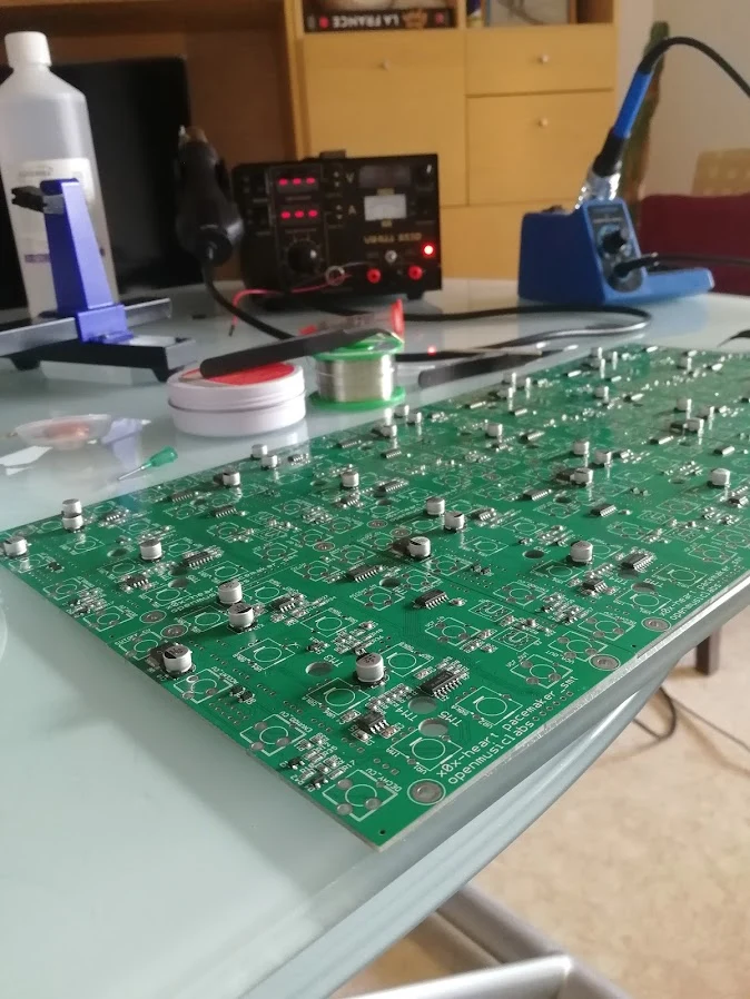
Crafting silicon

Why does everyone make them square?

MLIR

LLVM

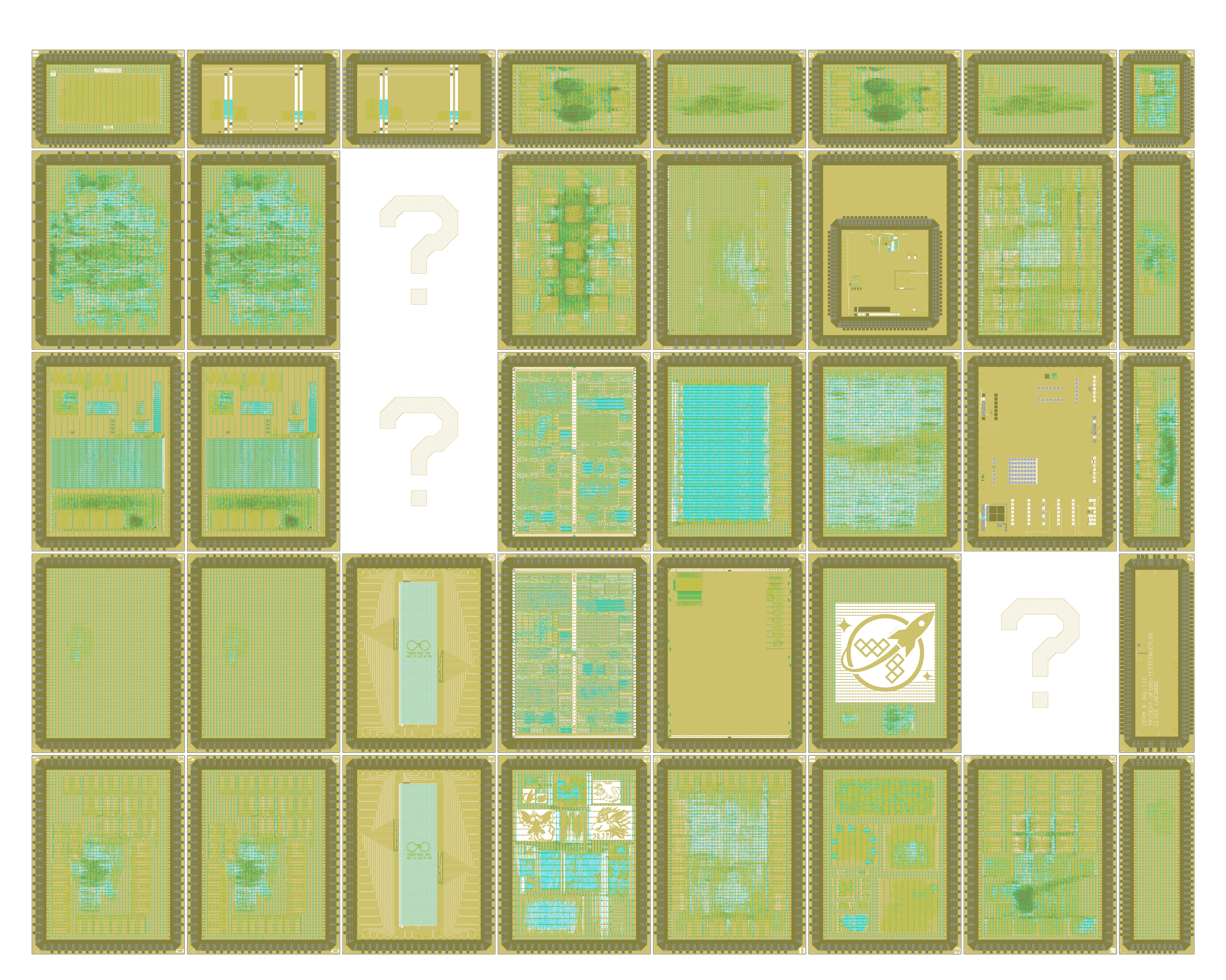
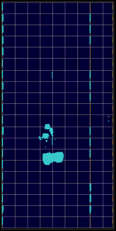
OpenROAD placement as a visual medium.

From problems to electron flow

From pressure to specialization

This section explains why modern compiler techniques must reach into hardware.

  1. Layers: follow arithmetic choices from programs toward circuits.

  2. Scaling limits: understand why performance no longer arrives for free.

  3. Specialization: connect GPUs, TPUs, and new number formats.

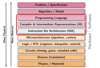
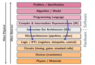
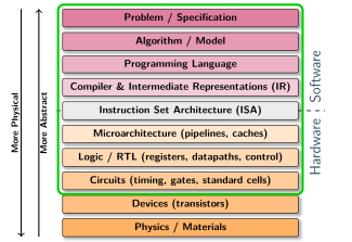
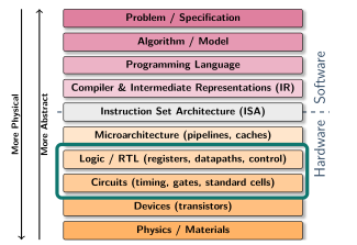
Arithmetic optimization spans the stack
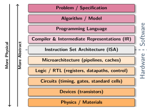
Computer-science abstraction layers from problem specification through software, hardware, devices, and physics Programming language, compiler IR, and ISA layers highlighted as the usual optimization window of a software compiler Arrows crossing the instruction-set boundary from compiler representations to hardware logic and RTL A large frame spanning abstraction layers from problem specification through circuits to represent MLIR's multi-level view Logic and RTL plus circuit layers highlighted as the focus of this course

One problem, many representations

  • Each layer exposes different decisions.

  • Software and hardware are intertwined and multi-level.

1. Optimize a fixed machine

  • Algebraic simplification: \(x \times 1 \rightarrow x\).

  • Strength reduction: \(x \times 2 \rightarrow x \ll 1\).

  • Instruction selection: fused multiply-add.

A compiler usually sees a local window.

2. Build the machine

  • High-level synthesis crosses the ISA boundary.

  • Specialize operators: \(x^2\), \(x/3\).

  • Fuse operators and map them to LUTs or DSPs.

More hardware freedom means more opportunities.

3. Traverse the stack

  • MLIR dialects keep domain intent explicit.

  • Lowerings connect many domain-specific representations.

  • One infrastructure can move from problem to circuit.

MLIR offers a larger view.

This presentation lives here!

  • Logic / RTL: hardware structure, datapaths, and state.

  • Circuits: Boolean networks, synthesis, and cost.

  • Hands-on: lower arithmetic operations into explicit circuits.

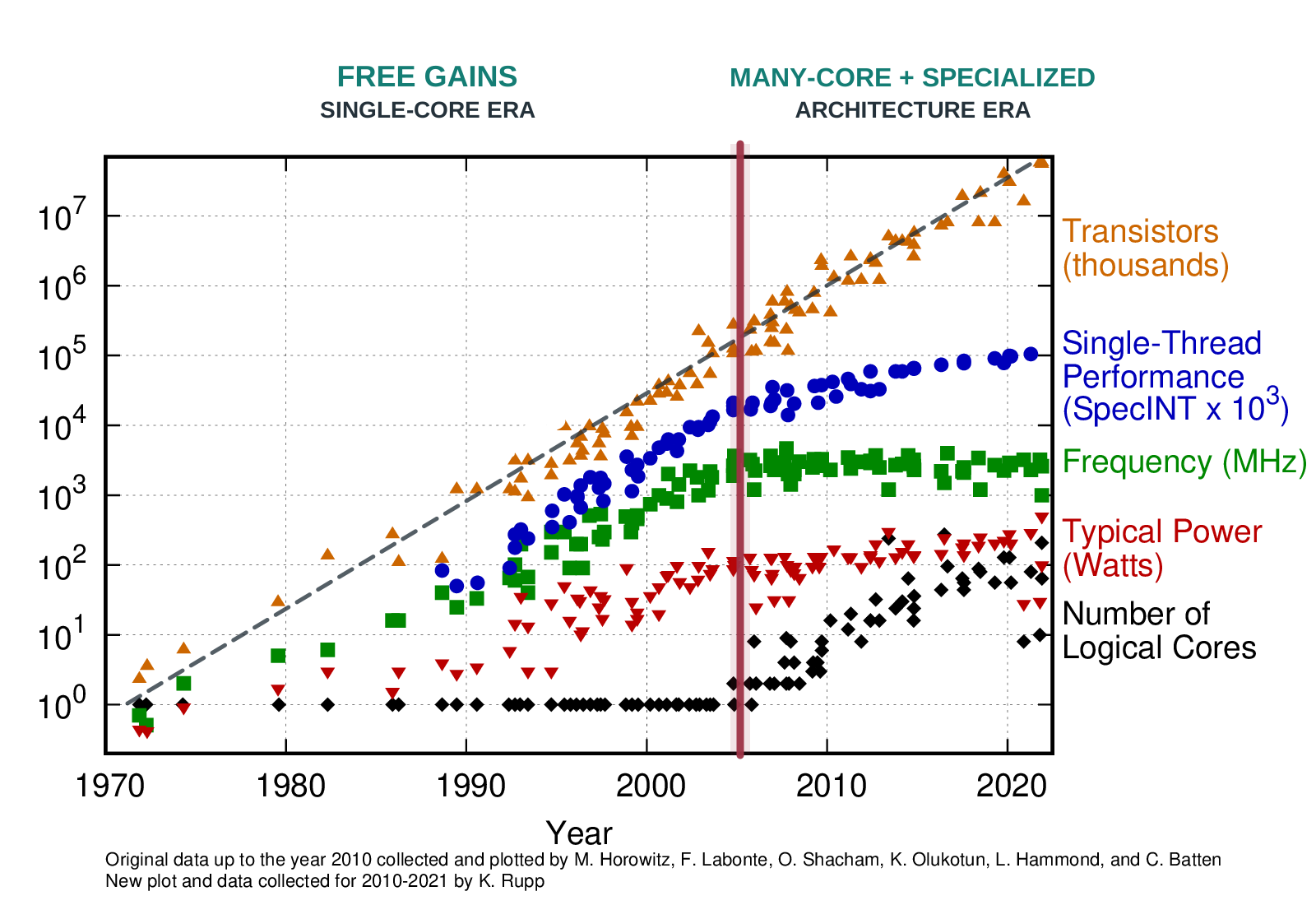
The free speedups ended
Quiz time

Who has seen a version of this plot before?

Karl Rupp's plot of transistor count, single-thread performance, frequency, power, and logical core count from 1970 to 2021, annotated with a Moore's law guide and a boundary between the single-core free-gains era and the many-core and specialized-architecture era

Fifty years of microprocessor trends. (Rupp 2022)

The free speedups ended

Karl Rupp's plot of transistor count, single-thread performance, frequency, power, and logical core count from 1970 to 2021, annotated with a Moore's law guide and a boundary between the single-core free-gains era and the many-core and specialized-architecture era

Fifty years of microprocessor trends. (Rupp 2022)

Quiz time

Who has heard these ADAges?

“Dark silicon era”

“Memory wall”

“Communication dominates arithmetic”

“End of the laws”

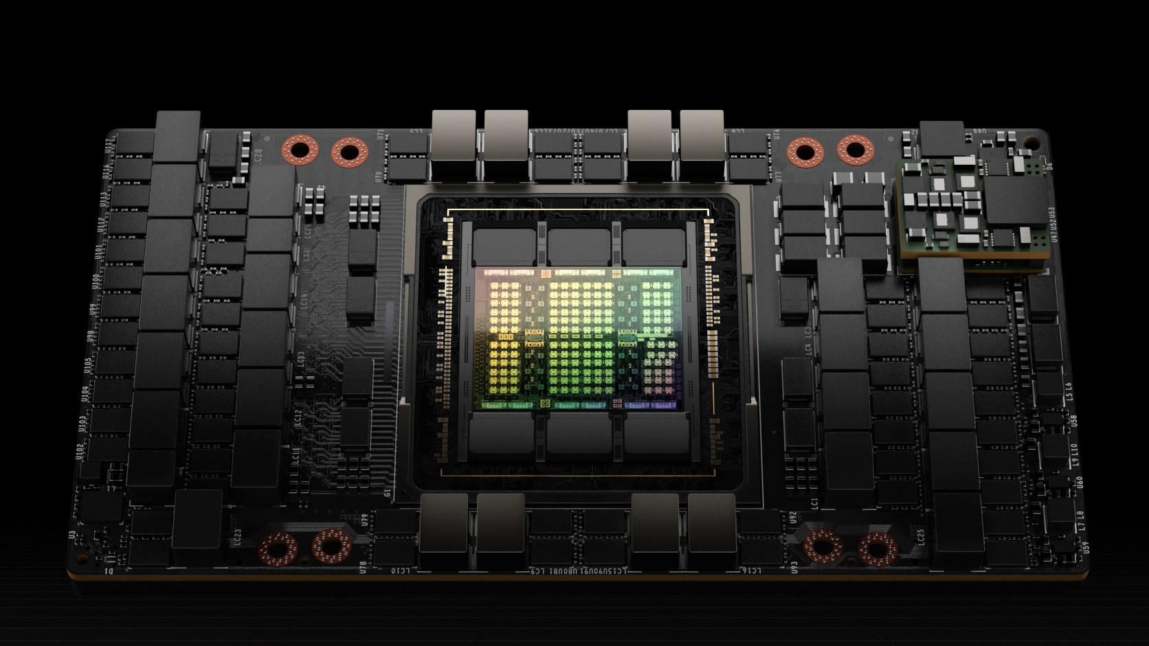
Some machines are experts at specialization
Quiz time

Who knows these machines?

NVIDIA H100 SXM5 GPU module with the central Hopper GPU and surrounding HBM stacks

GPU: matrix-multiply instructions backed by dedicated Tensor Core hardware. (NVIDIA 2022)
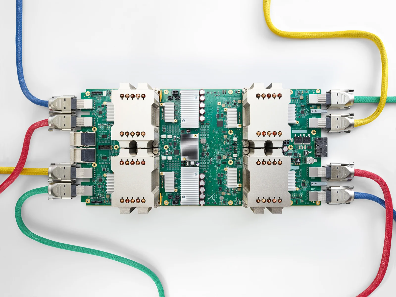
Google second-generation Cloud TPU board connected by colored high-speed interconnect cables

TPU: a processor built around matrix-multiply hardware. (Dean and Hölzle 2017; Jouppi et al. 2020)

Specialization puts more of the problem directly into the machine.

New accelerators, new compiler stacks: one origin of MLIR.

Digital design primer

The digital-design primer

These concepts become CIRCT vocabulary in the next section.

  1. Logic: combinational operations and bit widths.

  2. Time: registers, clocks, and timing.

  3. Structure: modules, instances, and repeated hardware.

  4. Targets: FPGA fabrics and ASIC geometry.

Quiz time

Quick show of hands

Who has already:

  • written VHDL;
  • written Verilog or SystemVerilog;
  • used an FPGA;
  • seen an ASIC design flow?

Essential follow-up

Who has never heard any of those words?

So I know exactly how much to panic.

We will use tiny SystemVerilog examples only to make the hardware visible.

Combinational logic

Question

Which line runs first?

module mul_add4(
  input  logic [3:0] a, b, c,
  output logic [8:0] d
);
  logic [7:0] product;

  assign d =
      {1'b0, product} + {5'b0, c};

  assign product =
      {4'b0, a} * {4'b0, b};
endmodule

Neither line runs first.

  • Both operators exist at the same time.
  • The adder output settles after product reaches it.
  • With no register, there is no stored state or clock cycle.

Compiler takeaway

Dependency analysis recovers the graph, independent of source order.

Bit widths: where does the carry go?

Question

For a = 15 and b = 1, what values reach wrapped and exact?

logic [3:0] a, b;
logic [3:0] wrapped;
logic [4:0] exact;

assign wrapped = a + b;
assign exact =
    {1'b0, a} + {1'b0, b};
wrapped = 4'b0000   // 0
exact   = 5'b10000  // 16

The carry exists only when the wires have room for it. Width is behavior.

Compiler takeaway

Range analysis can prove smaller widths and narrow the circuit.

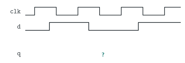
Registers: when does q change?

Question

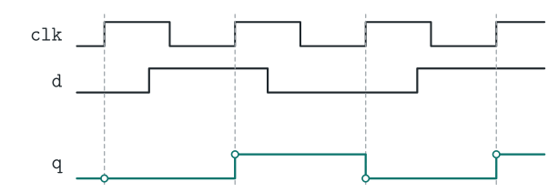
This register samples d on a rising edge. If d changes between two edges, when can q change?

Basic D-Q flip-flop: sample d on each rising edge.

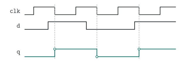
Falling-edge flip-flop: move the sampling instant.

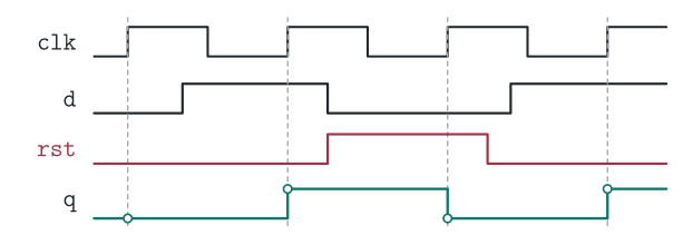
Synchronous reset: observe reset on the clock edge.

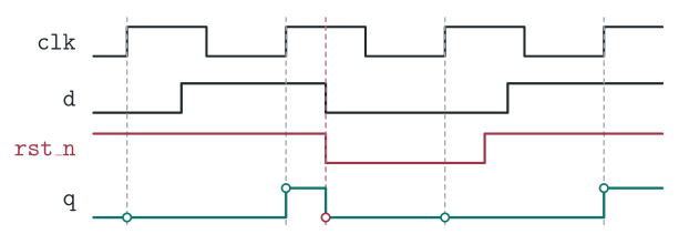
Asynchronous, active-low reset: reset immediately when rst_n falls.
always_ff @(posedge clk)
  q <= d;
// Basic D-Q Flip-Flop (FF).
always_ff @(posedge clk)
  q <= d;
// Falling-edge FF.
always_ff @(negedge clk)
  q <= d;
// Synchronous active-high reset.
always_ff @(posedge clk)
  if (rst) q <= 1'b0;
  else     q <= d;
// Asynchronous active-low reset.
always_ff @(posedge clk or negedge rst_n)
  if (!rst_n) q <= 1'b0;
  else        q <= d;

Timing diagram showing clock and d waveforms while the q waveform remains unknown

Completed timing diagram in which d changes between clock edges and q samples it only at rising edges

Timing diagram in which q samples d only at falling clock edges

Timing diagram in which an active-high synchronous reset changes q only at a rising clock edge

Timing diagram in which an active-low asynchronous reset changes q immediately when asserted

At the next rising edge. Between edges, q stores its previous value.

Changing posedge to negedge changes when the state may update.

Reset may assert between edges, but this flip-flop applies it only at the next rising edge.

Edge, reset timing, and reset polarity are hardware choices.

Compiler takeaway

Analyses can match these semantics to flip-flops in the target library.

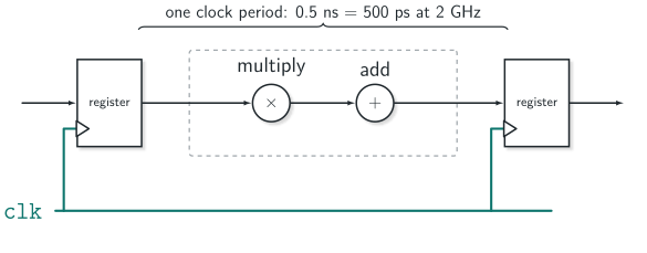
Clock quiz: what does 2 GHz mean?

Question

A processor is clocked at 2 GHz. How much time separates two rising edges?

\[ T = \frac{1}{f} = \frac{1}{2\,\text{GHz}} = 0.5\,\text{ns} = \mathbf{500\,\text{ps}} \]

Example cell delays

  • Sky130 HD OR2_1: 61 / 189 ps (rise / fall).
  • Kintex-7 LUT6: 119 ps (no routing).

Source register, combinational multiplier and adder, and destination register connected to a common clock

\[ t_{\text{clk} \rightarrow Q} + t_{\text{logic}} + t_{\text{routing}} + t_{\text{setup}} + t_{\text{skew}} < 500\,\text{ps} \]

The period is a budget for the longest register-to-register path.

Critical paths can be a compiler job

Compiler takeaway

Analyze the critical path \(\rightarrow\) insert registers \(\rightarrow\) balance stages.

Quiz: from function call to hardware

Question

Software calls a function. What is the equivalent mechanism in hardware?

Software: call a function. Hardware: instantiate a module.

// Declaration of a new module.
module mac4(
  input  logic [3:0] a, b, c,
  output logic [8:0] y
);
  logic [7:0] product;

  // Instantiation of an existing module.
  mul4 u_mul(
    .a(a), .b(b), .p(product));

  assign y =
    {1'b0, product} + {5'b0, c};
endmodule
// Declaration of a new module.
module mac4(
  input  logic [3:0] a, b, c,
  output logic [8:0] y
);
  logic [7:0] product;

  // Instantiation of an existing module.
  mul4 u_mul(
    .a(a), .b(b), .p(product));

  assign y =
    {1'b0, product} + {5'b0, c};
endmodule
  • mac4 becomes a reusable hardware definition.
  • u_mul names this instance of mul4.
  • Port connections become wires.

Quiz: one Processing Element (PE), or nine?

Question

Nine calls to one Processing Element (PE), or nine independent PEs?

genvar row, col;
generate
  for (row = 0; row < 3; row++)
    for (col = 0; col < 3; col++)
      pe u_pe(/* neighbours */);
endgenerate
genvar row, col;
generate
  for (row = 0; row < 3; row++)
    for (col = 0; col < 3; col++)
      pe u_pe(/* neighbours */);
endgenerate

Nine independent PEs, operating in parallel.

generate repeats structure during elaboration, before the circuit operates.
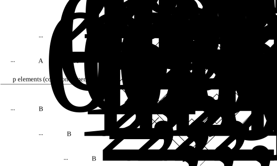
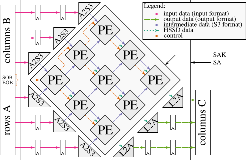
Three by three systolic array with nine processing elements and local diagonal data connections

3 \(\times\) 3 matrix-multiplication engine.

FPGA

Field-Programmable Gate Array

(the soft/easy hardware)

FPGA means configurable after manufacture
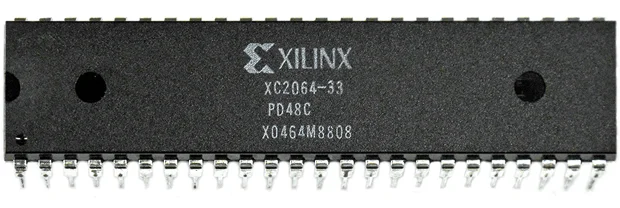
Xilinx XC2064 FPGA in a 48-pin dual in-line package

Xilinx XC2064 package.
  • 1985: Xilinx XC2064, the first commercial FPGA.
  • 128 LUTs: 64 logic blocks with two 3-input LUTs each.
  • Reconfigurable after manufacture.

Quiz: which function is in this LUT?
Question

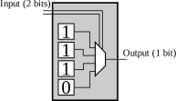
Which two-input gate is stored here?

Two input bits address one of four stored output bits in a lookup table

A 2-input lookup table.

Truth table

a b stored output
0 0 0
0 1 1
1 0 1
1 1 1

OR. A LUT2 stores \(2^2=4\) bits; a LUT6 stores \(2^6=64\) bits.

What if six inputs are not enough?

logic a, b, c, d, e, f, g;
logic y;

assign y = a | b | c | d |
           e | f | g;

Connect several LUTs. For example:

  1. one LUT computes a | b | c | d | e | f;
  2. another LUT combines that result with g.

Compiler takeaway

Technology mapping decomposes logic into target LUTs.

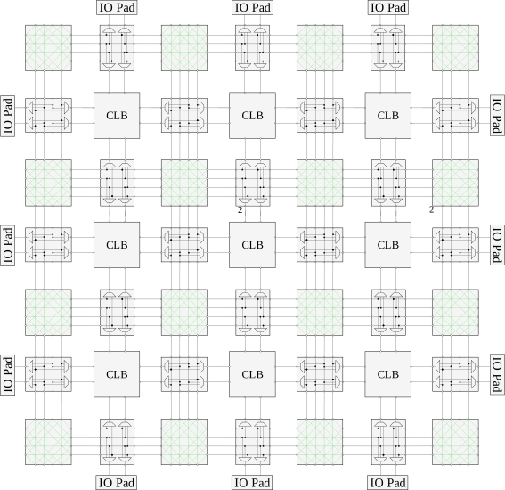
Many LUTs become one larger circuit

Island-style FPGA with configurable logic blocks, switch blocks, connection blocks, and IO pads

Simplified island-style FPGA architecture. (Ledoux 2024)
  • CLBs: groups of LUTs and flip-flops
  • Connection blocks: attach CLBs to routing tracks
  • Switch blocks: join the selected tracks
  • Hard blocks: DSPs and memories beside the fabric

Compiler takeaway

Synthesis decomposes the function, placement chooses the resources, and routing connects them into one circuit.

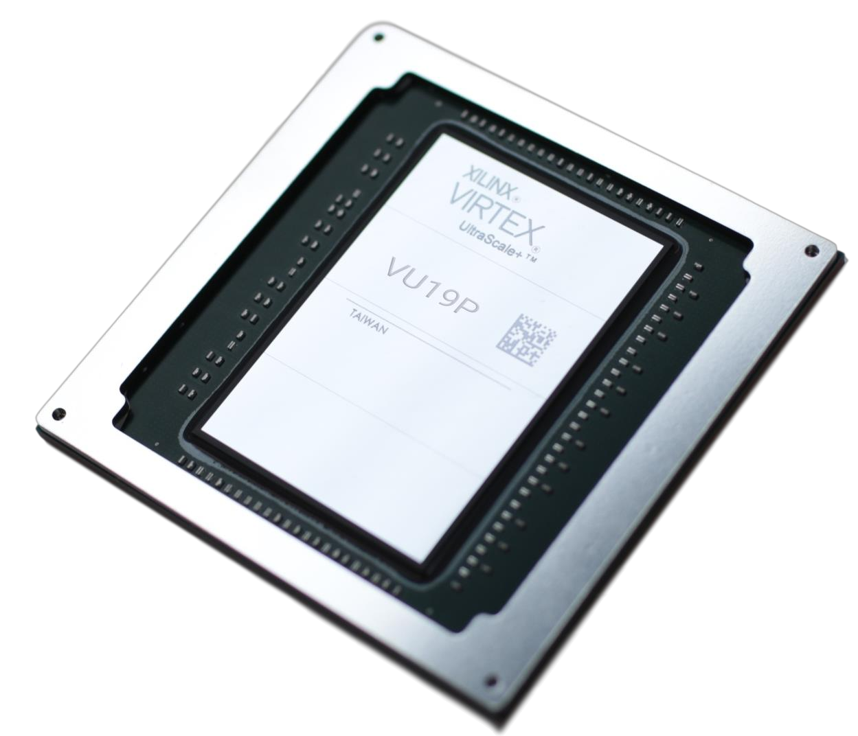
A modern FPGA is enormous

Large lidless Xilinx Virtex UltraScale Plus VU19P FPGA package

Xilinx Virtex UltraScale+ VU19P package. (Xilinx 2019)

Virtex UltraScale+ VU19P

  • 35 billion transistors
  • 9 million system logic cells
  • 2,072 user I/Os
  • 80 high-speed transceivers

Millions of configurable resources, memories, DSPs, and wires become the circuit described by one bitstream.

Compiler takeaway

Compilation can take several days.

ASIC

Application-Specific Integrated Circuit

(the hard hardware)

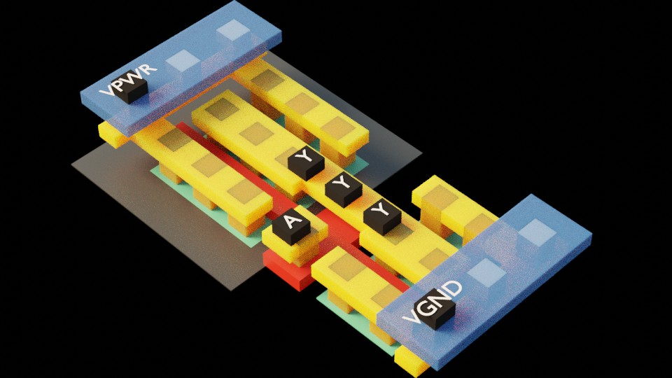
Quiz: what are we looking at?

Question

What hardware object is shown here?

Perspective rendering of an unlabelled SKY130 standard cell with input A, output Y, power, and ground pins

Look through the layers

Perspective rendering of a SKY130 standard cell

See? It kind of looks like this.

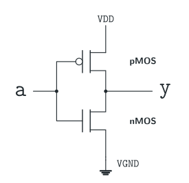
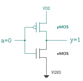
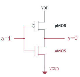
CMOS circuit with a pMOS above an nMOS transistor With input zero, the pMOS path drives the output high With input one, the nMOS path drives the output low

From geometry to logic (bottom-up)

Perspective rendering of a SKY130 inverter standard cell

SKY130 inv_2 render by Maximo Balestrini

CMOS implementation using one pMOS and one nMOS transistor

CMOS inverter: pMOS + nMOS

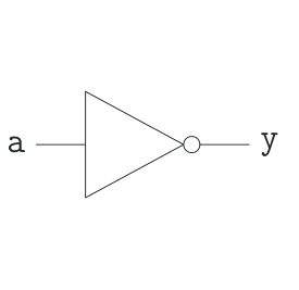
Logic symbol for an inverter with input a and output y

Inverter: y = ¬a

Yes: this line.

RTL

assign y = ~a;
  • Synthesis selects an inverter cell.
  • Physical design turns that cell into fixed polygons.

Later, the same in CIRCT:

%y = comb.xor %a, %one : i1

with %one = hw.constant true.

Perspective rendering of a SKY130 inverter standard cell selected for an RTL inversion

From RTL to GDSII

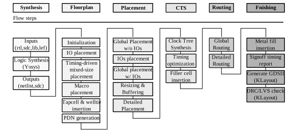
ASIC flow from synthesis through floorplanning, placement, clock-tree synthesis, routing, and GDSII generation

Main stages of an ASIC physical-design flow. (Ledoux 2024)
  1. Map RTL to logic cells.
  2. Floorplan and place them.
  3. Build the clock network.
  4. Route fixed metal wires.
  5. Verify and export GDSII.

RTL becomes geometry through a sequence of compiler passes and physical-design algorithms.

The best animation I have found for this part

Thumbnail for a Branch Education animation about transistors, logic gates, and CPU construction

How do Transistors Work? How are Transistors Assembled Inside a CPU?

I could add another 80 slides about fabrication. This 27-minute animation does it better.

If you want to build a real chip

Tiny Tapeout logo

Tiny Tapeout

Put a small design on a shared fabrication shuttle.

Zero to ASIC logo

Zero to ASIC

Learn the complete open-source digital ASIC flow.

They are friends: just knock on their doors. Cheap, modern paths to a real chip.

CIRCT: MLIR toward hardware

What is CIRCT?


TL;DR: Apply MLIR and LLVM compiler techniques to hardware-design tools.


CIRCT logo

Circuit IR Compilers and Tools

  • Recursively: CIRCT IR Compiler and Tools.
  • The T may be Tool, Translator, Team, Technology, Target, Tree, Type, …

Some other cool things:

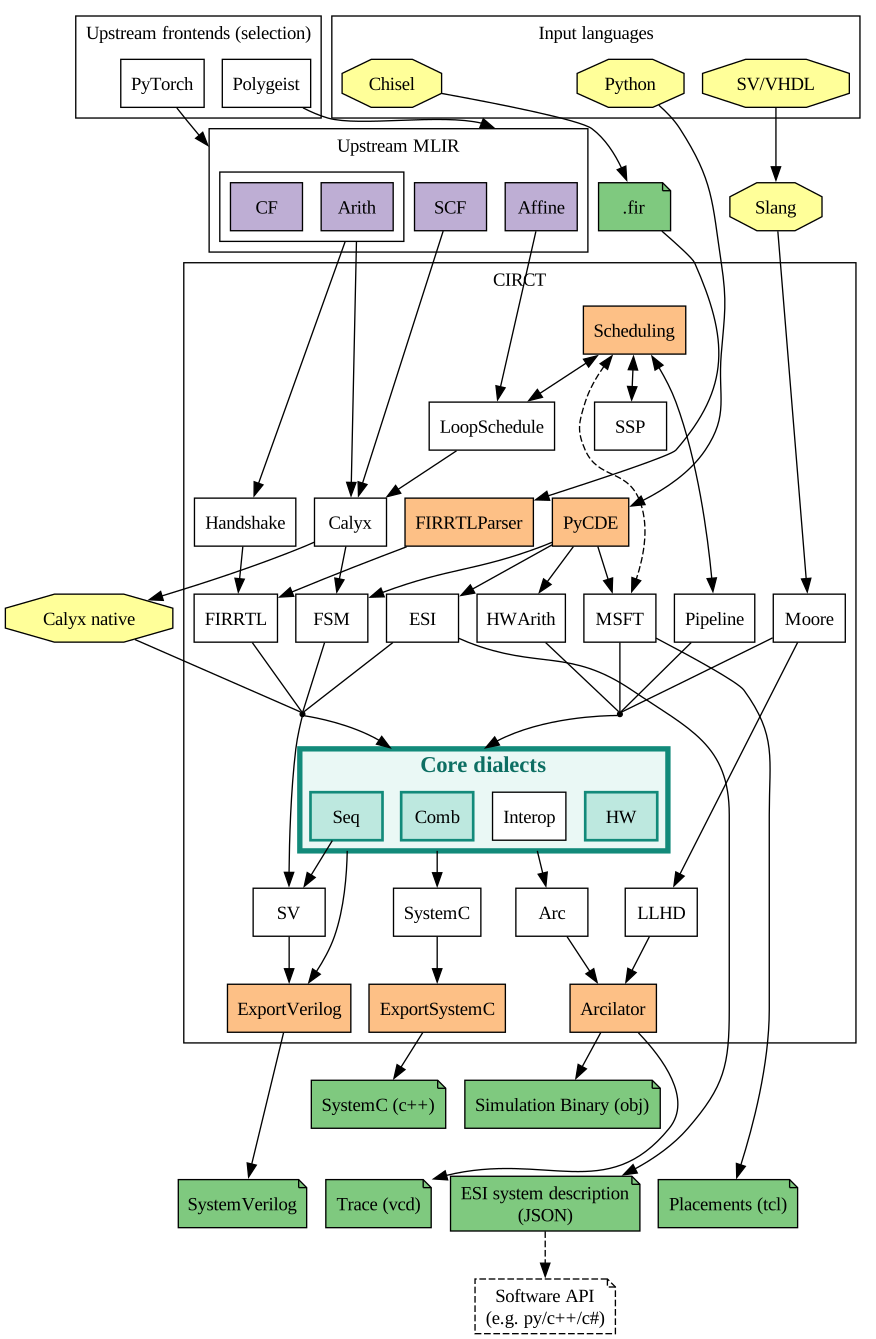
CIRCT defines the concepts from the primer


CIRCT Core:

  • hw: structure and hierarchy
  • comb: combinational logic
  • seq: registers and state


But also many other dialects:

  • Upstream MLIR: tensor, linalgfunc, scf, arith
  • Downstream: SystemVerilog → simulation, FPGA, ASIC tools

Next: use the CIRCT tools.
Overview of CIRCT with the core dialects highlighted

CIRCT dialect map. Source

CIRCT in practice

The CIRCT tool tour

This section follows the ARITH 2026 CIRCT Tutorial by Samuel Coward and me.

  1. Basics: circt-verilog, circt-opt, circt-lec, and firtool.

  2. Synthesis & Reports: circt-synth, AIGER export, and area estimation.

Compiler explorers

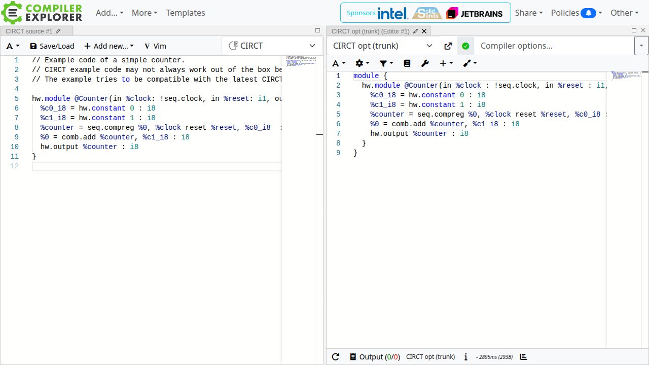
Compiler Explorer (Godbolt)

Compiler Explorer running CIRCT opt on a small CIRCT module

CIRCT IR \(\rightarrow\) circt-opt \(\rightarrow\) transformed IR

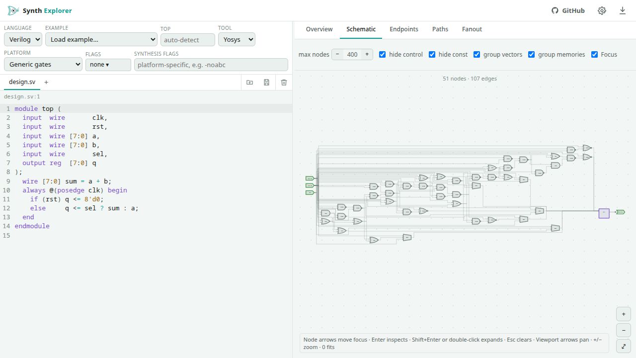
Synth Explorer

Synth Explorer showing Verilog beside its synthesized gate schematic

RTL \(\rightarrow\) Yosys or Vivado \(\rightarrow\) schematic

Tutorial Part 1: CIRCT basics

  • Exercise 1: Compile a SystemVerilog design to CIRCT IR. (\(\approx\) 3 min.)

  • Exercise 2: Narrow a combinational datapath with range analysis. (\(\approx\) 5 min.)

  • Exercise 3: Verify that a transformation preserved the circuit. (\(\approx\) 5 min.)

  • Exercise 4: Generate SystemVerilog for downstream EDA tools. (\(\approx\) 5 min.)

Exercise 1: compile the “FMA” example

First tool: circt-verilog parses SystemVerilog and prints CIRCT IR.

Let’s inspect the “FMA” module.

cat exercises/ex1_fma.sv


// exercises/ex1_fma.sv
module ex1_fma (
  input  wire [3:0] a,
  input  wire [3:0] b,
  input  wire [3:0] c,
  output wire [8:0] d
);
  assign d = (a * b) + (c * 1'd1);
endmodule

(SystemVerilog support remains an ongoing effort documented by Chips Alliance sv-tests.)

… and its MLIR/CIRCT counterpart

circt-verilog exercises/ex1_fma.sv


module {
  hw.module @ex1_fma(
      in %a : i4, in %b : i4, in %c : i4,
      out d : i9) {
    %c0_i5 = hw.constant 0 : i5
    %0 = comb.concat %c0_i5, %a : i5, i4
    %1 = comb.concat %c0_i5, %b : i5, i4
    %2 = comb.mul %0, %1 : i9
    %3 = comb.concat %c0_i5, %c : i5, i4
    %4 = comb.add %2, %3 : i9
    hw.output %4 : i9
  }
}

Exercise 1: compile the “FMA” example

// exercises/ex1_fma.sv
module ex1_fma (
  input  wire [3:0] a,
  input  wire [3:0] b,
  input  wire [3:0] c,
  output wire [8:0] d
);
  assign d = (a * b) + (c * 1'd1);
endmodule
module {
  hw.module @ex1_fma(
      in %a : i4, in %b : i4, in %c : i4,
      out d : i9) {
    %c0_i5 = hw.constant 0 : i5
    %0 = comb.concat %c0_i5, %a : i5, i4
    %1 = comb.concat %c0_i5, %b : i5, i4
    %2 = comb.mul %0, %1 : i9
    %3 = comb.concat %c0_i5, %c : i5, i4
    %4 = comb.add %2, %3 : i9
    hw.output %4 : i9
  }
}

Unlike C or SystemVerilog, comb does not implicitly promote arithmetic operands.

  • The operands and result of comb.mul and comb.add have the same width.

  • comb.concat makes each extension explicit in the IR.

  • A later analysis can therefore prove that those extra bits are unnecessary and narrow the circuit. (Exercise 2 ? Maybe ? Who knows ?)

Exercise 1: save the IR

Save the IR for Exercise 2:

circt-verilog exercises/ex1_fma.sv -o exercises/ex1_fma.mlir


  • Without -o, use the terminal to inspect a transformation immediately.
  • With -o, keep an intermediate representation for another pass or tool.
  • The file is text: inspect it with less, vim, or nano.

Exercise 2: find the redundant bit

Question

The imported IR uses i9 throughout the datapath. How many bits can these values actually require?

hw.module @ex1_fma(
    in %a : i4, in %b : i4, in %c : i4,
    out d : i9) {
  %c0_i5 = hw.constant 0 : i5
  %0 = comb.concat %c0_i5, %a : i5, i4
  %1 = comb.concat %c0_i5, %b : i5, i4
  %2 = comb.mul %0, %1 : i9
  %3 = comb.concat %c0_i5, %c : i5, i4
  %4 = comb.add %2, %3 : i9
  hw.output %4 : i9
}
Value Possible unsigned values Required width
%a, %b, %c \([0, 15]\) 4 bits
%a * %b \([0, 225]\) 8 bits
%a * %b + %c \([0, 240]\) 8 bits

The ninth bit belongs to the module interface, not to the internal arithmetic.

Exercise 2: read the narrowing contract

comb-int-range-narrowing makes that range argument mechanically:

def CombIntRangeNarrowing : Pass<"comb-int-range-narrowing"> {
  let summary = "Reduce comb op bitwidth based on integer range analysis.";
  let description = [{
    Compute a basic value range analysis, by propagating integer intervals
    through the domain.
    The analysis is limited by a lack of sign-extension operator in the comb
    dialect, leading to an over-approximation.
    Particularly for signed arithmetic, a single interval is often an
    over-approximation, a more precise analysis would require a union of
    intervals.
  }];
}

For this zero-extended datapath, one interval per SSA value is precise enough; the signed-arithmetic limitation does not apply yet.

CIRCT Comb/Passes.td, pinned firtool-1.147.0 source

Exercise 2: run a deliberate pipeline

circt-opt exercises/ex1_fma.mlir \
  --comb-int-range-narrowing \
  --canonicalize \
  -o exercises/ex2_fma_optimized.mlir

The order is intentional:

  1. Range narrowing rewrites operation widths and inserts comb.extract or comb.concat where narrow operations meet wider values.
  2. Canonicalization cleans up the redundant structure exposed by that rewrite.

Exercise 2: inspect the transformed IR

--comb-int-range-narrowing

hw.module @ex1_fma(
    in %a : i4, in %b : i4, in %c : i4,
    out d : i9) {
  %false = hw.constant false
  %c0_i5 = hw.constant 0 : i5
  %0 = comb.concat %c0_i5, %a : i5, i4
  %1 = comb.concat %c0_i5, %b : i5, i4
  %2 = comb.extract %0 from 0 : (i9) -> i8
  %3 = comb.extract %1 from 0 : (i9) -> i8
  %4 = comb.mul %2, %3 : i8
  %5 = comb.concat %false, %4 : i1, i8
  %6 = comb.concat %c0_i5, %c : i5, i4
  %7 = comb.extract %5 from 0 : (i9) -> i8
  %8 = comb.extract %6 from 0 : (i9) -> i8
  %9 = comb.add %7, %8 : i8
  %10 = comb.concat %false, %9 : i1, i8
  hw.output %10 : i9
}

+ --canonicalize

hw.module @ex1_fma(
    in %a : i4, in %b : i4, in %c : i4,
    out d : i9) {
  %false = hw.constant false
  %c0_i4 = hw.constant 0 : i4
  %0 = comb.concat %c0_i4, %a : i4, i4
  %1 = comb.concat %c0_i4, %b : i4, i4
  %2 = comb.mul %0, %1 : i8
  %3 = comb.concat %c0_i4, %c : i4, i4
  %4 = comb.add %2, %3 : i8
  %5 = comb.concat %false, %4 : i1, i8
  hw.output %5 : i9
}

Exercise 2: make pass ordering observable

Now reverse the two passes:

circt-opt exercises/ex1_fma.mlir \
  --canonicalize \
  --comb-int-range-narrowing \
  -o exercises/ex2_fma_variant.mlir

diff -u exercises/ex2_fma_optimized.mlir exercises/ex2_fma_variant.mlir

Before reading the diff: will the semantics change? Will the operation count change? What single extra pass would recover the first output?

Answer: the arithmetic still narrows to i8, but late narrowing inserts comb.extract and comb.concat operations after canonicalization has already finished. The semantics are unchanged, the IR is larger, and a final --canonicalize recovers the first output.

Exercise 3: do you trust the transformation?

Of course, you do not trust research tools.

And industrial tools are always exact, except when their documentation lists IEEE-754 partial compliance and deviations.

CIRCT lets us mark our own homework with a logical equivalence checker: circt-lec.

Exercise 3: verify with circt-lec

General form:

circt-lec --c1 <module_1> <design_1.mlir> \
          --c2 <module_2> <design_2.mlir>


Our FMA:

circt-lec --c1 ex1_fma exercises/ex1_fma.mlir \
          --c2 ex1_fma exercises/ex2_fma_optimized.mlir


We should see:

c1 == c2

Exercise 3: how does circt-lec work?
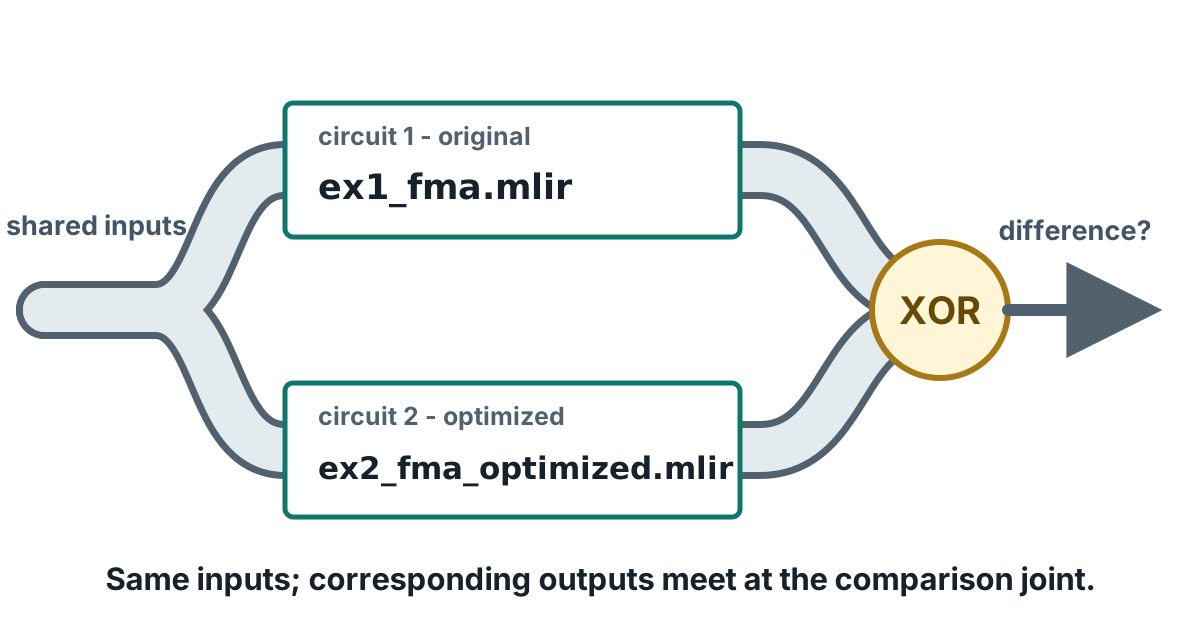
Quiz time

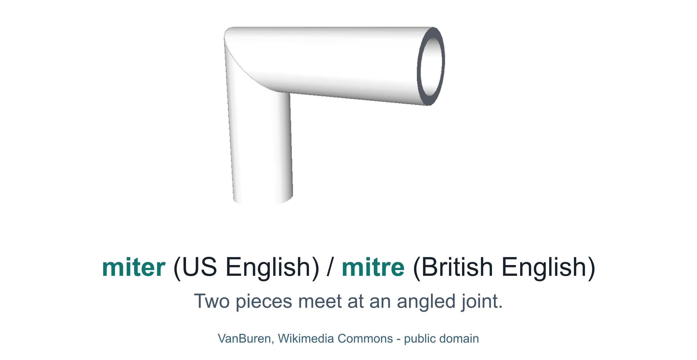
Who knows what a miter is?

An ordinary pipe miter or mitre joint

Shared inputs branching through ex1_fma and ex2_fma_optimized before their outputs meet at an XOR comparison joint

  1. Construct a circuit miter: drive both circuits with the same inputs and compare their outputs.

  2. Lower the miter and both circuits to SMT: Satisfiability Modulo Theories.

  3. Ask Z3 (an SMT solver) whether an input can make the outputs differ. unsat means there is no counterexample: c1 == c2.

  4. For our small circuits: same or not same :)

Exercise 3: break the circuit - 5 min

Introduce a functional bug while keeping the circuit valid and compilable. Then check that circt-lec reports c1 != c2.

cp exercises/ex2_fma_optimized.mlir exercises/ex3_fma_broken.mlir
nano exercises/ex3_fma_broken.mlir

circt-lec --c1 ex1_fma exercises/ex1_fma.mlir \
          --c2 ex1_fma exercises/ex3_fma_broken.mlir


Answer: Change the multiply to an add, alter a constant, or disconnect an operand. The current tool reports inequivalence but does not conveniently print the counterexample.

Exercise 4: generate SystemVerilog with firtool

A useful CIRCT flow is:

  1. Parse a SystemVerilog design into CIRCT IR.
  2. Optimize it with circt-opt and verify the transformations.
  3. Emit Verilog with firtool for downstream FPGA or ASIC tools.
firtool exercises/ex2_fma_optimized.mlir

exercises/ex2_fma_optimized.mlir is the output saved in Exercise 2.

module ex1_fma(
  input  [3:0] a, b, c,
  output [8:0] d
);
  assign d = {1'h0,
    {4'h0, a} * {4'h0, b} + {4'h0, c}};
endmodule

Exercise 4: verify the round trip - 5 min

  1. Modify the firtool command to save the generated Verilog.
  2. Compile that Verilog back to CIRCT IR with circt-verilog.
  3. Use circt-lec to prove that the round trip preserved equivalence.
firtool exercises/ex2_fma_optimized.mlir -o exercises/ex4_fma_roundtrip.sv
circt-verilog exercises/ex4_fma_roundtrip.sv -o exercises/ex4_fma_roundtrip.mlir
circt-lec --c1 ex1_fma exercises/ex2_fma_optimized.mlir \
          --c2 ex1_fma exercises/ex4_fma_roundtrip.mlir

Tutorial Part 2: synthesis and reports

AIGs · equivalence · structural cost

Synthesis: from comb to an AIG

hw + comb \(\xrightarrow{\texttt{circt-synth}}\) synth.aig + reports

Logic synthesis lowers adders, muxes, and other operations into Boolean logic, then simplifies and shares that logic.

An And-Inverter Graph (AIG) contains:

  • two-input AND vertices;
  • edges that may invert their value;
  • graph inputs and outputs.
%and = synth.aig.and_inv %a, %b : i1
%a_n_b = synth.aig.and_inv not %a, %b : i1

AND and inversion are sufficient because, for example,

\[a \lor b = \neg(\neg a \land \neg b).\]

The synth dialect represents the graph. AIGER is only a file format used to exchange it. (Mishchenko et al. 2006)

Exercise 5: simplify and measure - 12 min

Starting point

// exercises/ex5_aig.sv
always_comb begin
  out = a ? (b ? -x : -(x + 8'd1))
          : (b ? x + 8'd1 : x);
end

All operations are modulo \(2^8\).

Create exercises/ex5_aig_optimized.sv with the same module name and ports.

Measure the baseline

circt-verilog exercises/ex5_aig.sv \
  -o exercises/ex5_aig.mlir
circt-synth exercises/ex5_aig.mlir --top=ex5_aig \
  --analysis-output=exercises/ex5-reports \
  -o exercises/ex5_aig_synth.mlir

Baseline: 149 AIG nodes · 13 logic levels

Task: preserve c1 == c2, but build a smaller and shallower AIG.

Exercise 5: simplify the four cases

All arithmetic is eight-bit modulo \(2^8\):

\[ -(x + 1) = \mathord{\sim}x \qquad -x = \mathord{\sim}x + 1 \]

Apply these identities to the two negative rows.

Original table

a b out
0 0 x
0 1 x + 1
1 0 -(x + 1)
1 1 -x

Simplified table

a b out
0 0 x
0 1 x + 1
1 0 ~x
1 1 ~x + 1

Question

Which input selects x or ~x? Which input selects +0 or +1?

Exercise 5: combine the controls

Simplified behavior

a b out
0 0 x
0 1 x + 1
1 0 ~x
1 1 ~x + 1

Question

How can a select x or ~x, while b selects +0 or +1?

1. Replicate a into an eight-bit mask

{8{a}} is 8'b00000000 when a = 0, and 8'b11111111 when a = 1.

2. Use XOR to select x or ~x

base = x ^ {8{a}}

3. Let b add zero or one

out = base + b

// solutions/ex5_aig_optimized.sv
assign out = (x ^ {8{a}}) + b;

Exercise 5: compare both designs

Import your implementation, then check equivalence and measure both AIGs:

circt-verilog exercises/ex5_aig_optimized.sv \
  -o exercises/ex5_aig_optimized.mlir

./scripts/compare-aig.py \
  exercises/ex5_aig.mlir \
  exercises/ex5_aig_optimized.mlir \
  ex5_aig
c1 == c2

AIG nodes       149 -> 54
logic levels     13 -> 8

The optimization removes 95 AIG nodes and 5 logic levels without changing the function.

Let’s multiply

“Be fruitful, and multiply.”

Genesis 1:28

What we will build

Until now, we used existing CIRCT passes. Now we write a lowering.

arith.mulf : f8E4M3FN \(\longrightarrow\) Python rewrite \(\longrightarrow\) hw + comb circuit

  1. Exercise 6 — warm-up: go from upstream func + arith MLIR to a hardware circuit.

  2. Exercise 7 — build: construct and test an E4M3 multiplier datapath.

  3. Exercise 8 — specialize (optional): detect x * x and generate a cheaper squarer.

Exercise 6: from upstream MLIR to a circuit

cat exercises/ex6_arith_muli.mlir
module {
  func.func @ex6_mul(%a : i8, %b : i8) -> i8 {
    %r = arith.muli %a, %b : i8
    return %r : i8
  }
}

Objective: a combinational hardware module

hw.module @ex6_mul(
    in %in0 : i8, in %in1 : i8, out out0 : i8) {
  %0 = comb.mul %in0, %in1 : i8
  hw.output %0 : i8
}

This is the smallest complete path to SystemVerilog and logic synthesis.

Exercise 6: find the missing passes - 3 min

To reach that objective, two things must change:

  • func.func and return must become a hardware module boundary.
  • arith.muli must become a combinational multiplier.

Does upstream circt-opt provide both transformations?

circt-opt --help | grep -i arith
circt-opt --help | grep -i func

Relevant arith result

--convert-comb-to-arith
--lower-hwarith-to-hw
--map-arith-to-comb

Relevant func result

--lower-cf-to-handshake
    Lower func and CF into Handshake IR

No direct generic func.funchw.module pass.

Exercise 6: compose two passes

circt-tutorial-opt exercises/ex6_arith_muli.mlir \
  --tutorial-func-to-hw -o exercises/ex6_hw_arith.mlir

circt-opt exercises/ex6_hw_arith.mlir \
  --map-arith-to-comb -o exercises/ex6_hw_comb.mlir
File Boundary Multiplication
ex6_arith_muli.mlir func.func arith.muli
ex6_hw_arith.mlir hw.module arith.muli
ex6_hw_comb.mlir hw.module comb.mul

Boundary first; multiplication second.

MLIR 2 SV 2 GDS in seconds :)

  1. This you know: get SystemVerilog from MLIR with firtool.
firtool exercises/ex6_hw_comb.mlir -o exercises/ex6_mul.sv
  1. Copy the RTL and run OpenROAD to get a Sky130 GDSII.
cp exercises/ex6_mul.sv \
  ~/Documents/work/repositories/OpenROAD-flow-scripts-feature-sonification/flow/designs/src/ex6_mul/
cd ~/Documents/work/repositories/OpenROAD-flow-scripts-feature-sonification/flow
make DESIGN_CONFIG=designs/sky130hd/ex6_mul/config.mk
  1. Open the 3D viewer and drop the generated layout into it.
r
cd tinytapeout_gds_viewer
npm start
firefox http://localhost:5173/
~/Documents/work/repositories/OpenROAD-flow-scripts-feature-sonification/flow/results/sky130hd/ex6_mul/base/6_final.gds

Exercise 6: change the arithmetic contract

module {
  func.func @ex6_mul(%a : f8E4M3FN, %b : f8E4M3FN) -> f8E4M3FN {
    %r = arith.mulf %a, %b : f8E4M3FN
    return %r : f8E4M3FN
  }
}

Run the same two-stage pipeline on exercises/ex6_arith_mulf.mlir:

circt-tutorial-opt exercises/ex6_arith_mulf.mlir \
  --tutorial-func-to-hw -o exercises/ex6_float_hw_arith.mlir
circt-opt exercises/ex6_float_hw_arith.mlir --map-arith-to-comb
error: failed to legalize operation 'arith.mulf'

map-arith-to-comb draws a deliberate line

def MapArithToCombPass : Pass<"map-arith-to-comb"> {
  let summary = "Map arith ops to combinational logic";
  let description = [{
    A pass which does a simple `arith` to `comb` mapping wherever possible.
    This pass will not convert:
    * floating point operations
    * operations using `vector`-typed values

    This does not intend to be the definitive lowering/HLS pass of `arith`
    operations in CIRCT (hence the name "map" instead of e.g. "lower").
    Rather, it provides a simple way (mostly for testing purposes) to map
    `arith` operations.
  }];
}

CIRCT Transforms/Passes.td, pinned firtool-1.147.0 source

The failure is the documented boundary of the pass. Our exercise supplies one concrete floating-point lowering.

Read the type name: f8E4M3FN

Part Meaning
f8 8-bit floating-point type
E4 4 exponent bits
M3 3 stored mantissa/fraction bits
FN F = finite; N = NaN. No infinity encoding.

Overflow therefore produces NaN instead of infinity.

MLIR Builtin floating-point types

Eight bits encode several numerical regimes

s

[7]

sign · 1 bit

eeee

[6:3]

biased exponent · 4 bits

mmm

[2:0]

stored fraction · 3 bits

Regime Encoding Value
zero e = 0000, m = 000 \(0\)
subnormal e = 0000, m != 000 \((-1)^s 2^{-6}(m/8)\)
normal e != 0000 \((-1)^s 2^{e-7}(1+m/8)\)
NaN e = 1111, m = 111 not a number

f8E4M3FN has bias 7, finite values up to 448, and no infinity. (Micikevicius et al. 2022)

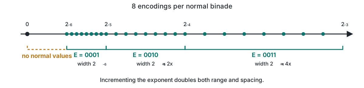
Why subnormal values?

You may remember binary scientific notation:

  • Normal: normalized binary scientific notation, \(1.mmm_2 \times 2^e\).
  • At \(e_{\min}=-6\), no smaller exponent exists; without subnormals, the next representable value below \(2^{-6}\) is zero.

Subnormal: keep \(e=-6\) and allow \(0.mmm_2 \times 2^{-6}\); seven values fill the gap gradually.
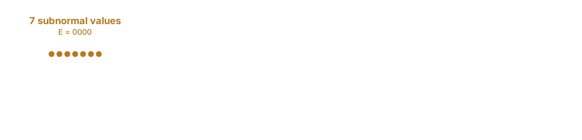
Normal E4M3FN binades double in width and leave no normal values between zero and two to the minus six

Seven subnormal values fill the interval next to zero

Exercise 7: exact normal finite products only.

Set aside: zero, subnormals, NaNs, overflow/underflow, and rounding.

All 256 E4M3FN encodings
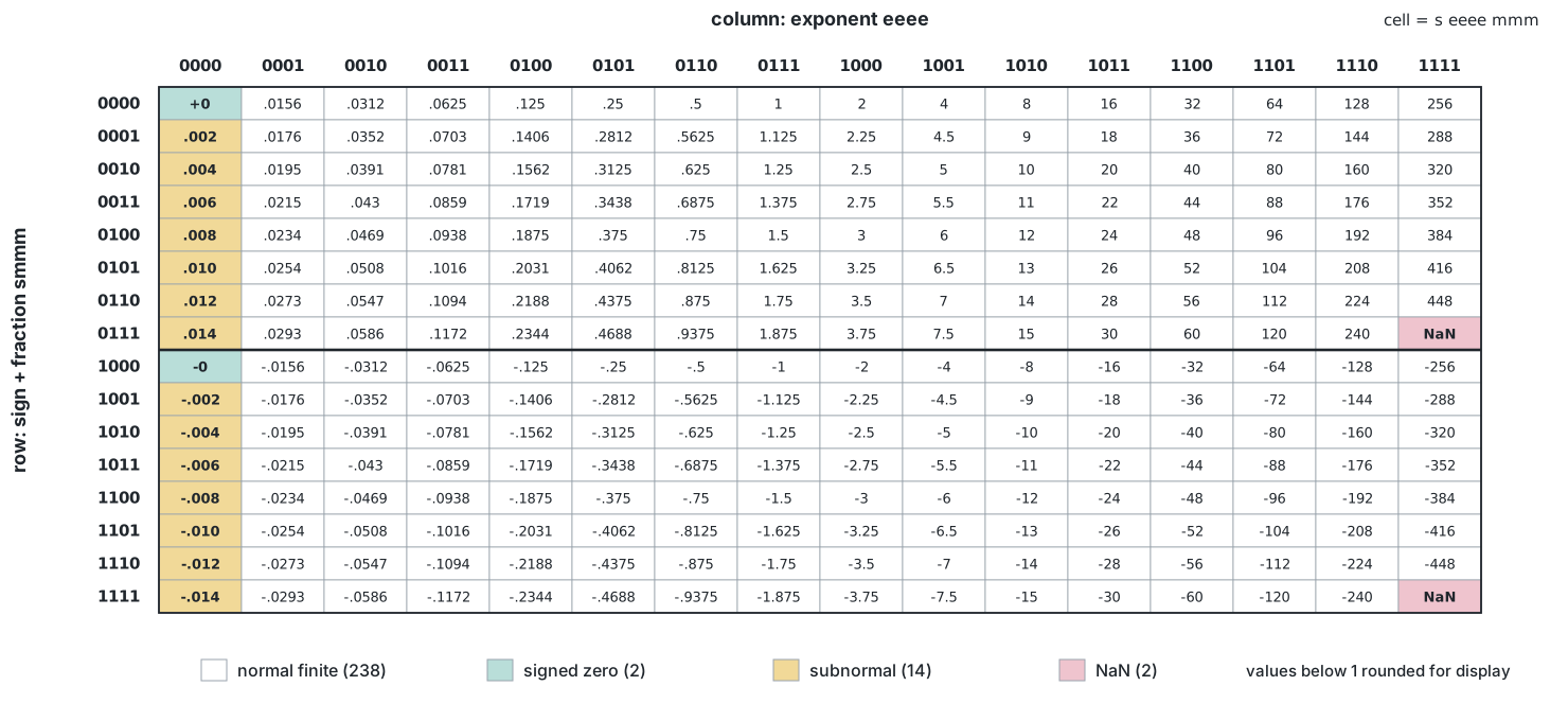
Table of all 256 E4M3FN values with exponent bits from 0000 to 1111 across columns and sign plus fraction bits from 0000 to 1111 across rows; zeros, subnormals, and NaNs are colorized

Exercise cheat sheet

I need to… Use
Edit locally; run in Docker docker run -it -v "$PWD:/workspace" ghcr.io/bynaryman/mlir-summer-school-2026-circt:latest
Build and run the supplied pipeline ./scripts/build.sh && ./scripts/run.sh
SystemVerilog -> MLIR circt-verilog in.sv -o out.mlir
Apply passes circt-opt in.mlir --PASS -o out.mlir
MLIR -> SystemVerilog firtool in.mlir -o out.sv
Prove equivalent circt-lec --c1 TOP before.mlir --c2 TOP after.mlir
Compare synthesis statistics ./scripts/compare-aig.py BEFORE.mlir AFTER.mlir TOP
Run the Python lowering python scripts/lower-e4m3fn.py in.mlir -o out.mlir
Create XOR x = comb.XorOp.create(a, b).result
Replace an operation rewriter.replace_op(op, [value])
Test the E4M3 normal path ./scripts/test-e4m3-all.py --pass --normal-path

Exercise 7: build an E4M3 multiplier
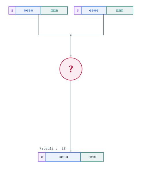
Two E4M3 inputs above an empty vertical multiplier datapath and an eight-bit result Two E4M3 inputs joining at a question mark before an E4M3 result

Input excerpt: exercises/ex7_e4m3fn_mul.mlir

%af = arith.bitcast %a : i8 to f8E4M3FN
%bf = arith.bitcast %b : i8 to f8E4M3FN
%product = arith.mulf %af, %bf : f8E4M3FN
%result = arith.bitcast %product : f8E4M3FN to i8

Root the rewrite at the final arith.bitcast: the matched island and its replacement then have the same i8 boundary.

Pass skeleton: scripts/lower-e4m3fn.py

def lower_e4m3_mul(out_cast, rewriter):
    matched = match_e4m3_island(out_cast)  # supplied
    if matched is None:
        return True
    lhs, rhs = matched
    with rewriter.ip:
        ...
    rewriter.replace_op(out_cast, [result])
    return False

patterns.add(
    arith.BitcastOp, lower_e4m3_mul)

Supplied: matcher and integer type aliases · API: official CIRCT Python bindings · Scope: exact normal finite products; no rounding.

What must the circuit compute?

Two E4M3 inputs above an empty multiplier datapath Unknown E4M3 multiplier implementation

For a normal, finite value, let \(E\) be the stored exponent, \(B=7\), and \(M\) the significand:

\[x=\color{#7c3aed}{(-1)^s}\, \color{#2563eb}{2^{E-B}}\, \color{#0f766e}{M}, \qquad \color{#0f766e}{M=(1.\mathtt{mmm})_2}\]

Multiplying two values exposes the three datapaths we must build:

\[ab= \color{#7c3aed}{\underbrace{(-1)^{s_a\oplus s_b}}_{\text{sign}}} \;\color{#2563eb}{\underbrace{2^{(E_a-B)+(E_b-B)}}_{\text{exponent}}} \;\color{#0f766e}{\underbrace{(M_aM_b)}_{\text{significand}}}\]

The significand product may need normalization; that correction is then added to the result exponent.

Together: route the sign
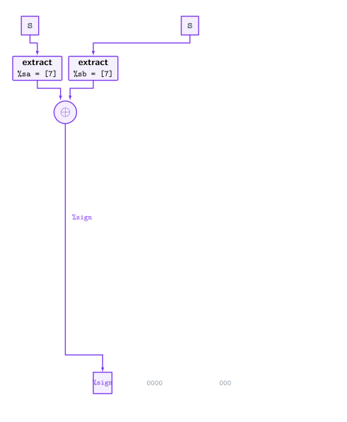
E4M3 multiplier datapath

First: compute the sign.

\[(-1)^{s_a}(-1)^{s_b}=(-1)^{s_a+s_b} \quad\Longrightarrow\quad s_r=s_a\oplus s_b\]

First make the rewrite compile. Extract both signs, XOR them, and set the remaining seven output bits to zero.

Sign path

sa = comb.ExtractOp.create(7, i1, lhs).result
sb = comb.ExtractOp.create(7, i1, rhs).result
sign = comb.XorOp.create(sa, sb).result

zero7 = hw.ConstantOp.create(i7, 0).result
result = comb.ConcatOp.create(sign, zero7).result

The long purple wire is now a real SSA value from both inputs to the packed result.

Solution checkpoint: sign

Cumulative schematic

E4M3 multiplier datapath

def lower_e4m3_mul(out_cast, rewriter):
    matched = match_e4m3_island(out_cast)
    if matched is None:
        return True
    lhs, rhs = matched
    with rewriter.ip:
        sa = comb.ExtractOp.create(7, i1, lhs).result
        sb = comb.ExtractOp.create(7, i1, rhs).result
        sign = comb.XorOp.create(sa, sb).result
        zero7 = hw.ConstantOp.create(i7, 0).result
        result = comb.ConcatOp.create(sign, zero7).result
    rewriter.replace_op(out_cast, [result])
    return False

Exercise 7A: multiply the significands - 6 min
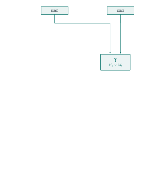
E4M3 multiplier with its sign path completed The significand product is the next datapath to implement

Now: multiply the significands.

Normalized scientific notation keeps one non-zero digit before the point. In binary that digit can only be 1, so every normal significand is 1.mmm₂. Because this leading 1 is predictable, E4M3 stores only mmm.

\[M=1+\frac{(\mathtt{mmm})_2}{2^3}=(1.\mathtt{mmm})_2, \qquad \boxed{P=M_aM_b}\]

Your step: prepend the implicit 1, form both 4-bit significands, then produce the full-width %product : i8. comb.mul returns the operand width.

Exercise 7A: solution
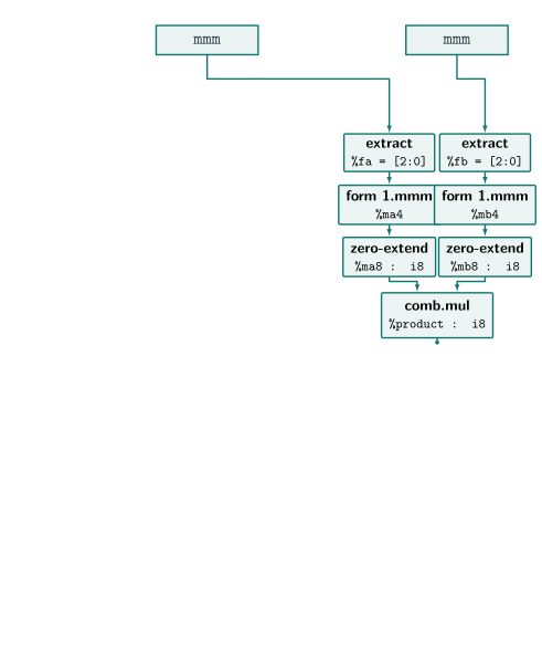
E4M3 multiplier with its significand product completed

Now: multiply the significands.

Reconstruct 1.mmm₂, zero-extend both 4-bit significands to the result width, then multiply them as integers.

\[M=1+\frac{(\mathtt{mmm})_2}{2^3}=(1.\mathtt{mmm})_2, \qquad P=M_aM_b\]

Solution

fa = comb.ExtractOp.create(0, i3, lhs).result
fb = comb.ExtractOp.create(0, i3, rhs).result
one = hw.ConstantOp.create(i1, 1).result
ma4 = comb.ConcatOp.create(one, fa).result
mb4 = comb.ConcatOp.create(one, fb).result
zero4 = hw.ConstantOp.create(i4, 0).result
ma8 = comb.ConcatOp.create(zero4, ma4).result
mb8 = comb.ConcatOp.create(zero4, mb4).result
product = comb.MulOp.create(ma8, mb8).result

Solution checkpoint: significand

Cumulative schematic

E4M3 multiplier with its significand product completed

def lower_e4m3_mul(out_cast, rewriter):
    matched = match_e4m3_island(out_cast)
    if matched is None:
        return True
    lhs, rhs = matched
    with rewriter.ip:
        sa = comb.ExtractOp.create(7, i1, lhs).result
        sb = comb.ExtractOp.create(7, i1, rhs).result
        sign = comb.XorOp.create(sa, sb).result
        fa = comb.ExtractOp.create(0, i3, lhs).result
        fb = comb.ExtractOp.create(0, i3, rhs).result
        one = hw.ConstantOp.create(i1, 1).result
        ma4 = comb.ConcatOp.create(one, fa).result
        mb4 = comb.ConcatOp.create(one, fb).result
        zero4 = hw.ConstantOp.create(i4, 0).result
        ma8 = comb.ConcatOp.create(zero4, ma4).result
        mb8 = comb.ConcatOp.create(zero4, mb4).result
        product = comb.MulOp.create(ma8, mb8).result
        zero7 = hw.ConstantOp.create(i7, 0).result
        result = comb.ConcatOp.create(sign, zero7).result
    rewriter.replace_op(out_cast, [result])
    return False

Exercise 7B: normalize the product - 7 min

E4M3 multiplier through the full significand product

Next: normalize the product.

ma4 and mb4 encode 1.mmm₂: four stored bits with three fractional positions. Their eight-bit integer product therefore has six fractional positions; the binary point is implicit, not stored.

Stored %product : i8 Test Keep Exponent
01xxxxxx₂ %product[7] = 0 %product[6:3] + 0
1xxxxxxx₂ %product[7] = 1 %product[7:4] + 1
Product: stored bits (UQ2.6) Decimal Shift
1100 × 1000 = 01100000 (01.100000) 1.5 no
1100 × 1100 = 10010000 (10.010000) 2.25 yes
1111 × 1111 = 11100001 (11.100001) 3.515625 yes

%product[7] is 1 when the product is greater than or equal to \(2\), outside the normalized significand interval \([1,2)\). Selecting the upper four bits divides it by two; incrementing the exponent preserves the value.

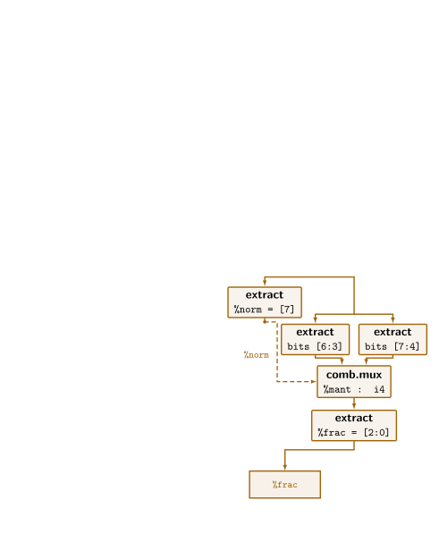
Your step: extract both four-bit windows, select one with %product[7], produce %frac : i3, and retain that bit as %norm : i1 for the exponent.

Exercise 7B: solution

E4M3 multiplier with normalization completed

\[n=\begin{cases}0 & P<2\\1 & P\ge 2\end{cases} \qquad M_r=P\,2^{-n}\]

%product[7] = 0 keeps %product[6:3]; %product[7] = 1 keeps %product[7:4]. Retain that same bit as the exponent correction.

Solution

norm = comb.ExtractOp.create(7, i1, product).result
direct = comb.ExtractOp.create(3, i4, product).result
shifted = comb.ExtractOp.create(4, i4, product).result
mant = comb.MuxOp.create(
    norm.value, shifted.value, direct.value).result
frac = comb.ExtractOp.create(0, i3, mant).result

Solution checkpoint: normalization

Cumulative schematic

E4M3 multiplier with normalization completed

def lower_e4m3_mul(out_cast, rewriter):
    matched = match_e4m3_island(out_cast)
    if matched is None:
        return True
    lhs, rhs = matched
    with rewriter.ip:
        sa = comb.ExtractOp.create(7, i1, lhs).result
        sb = comb.ExtractOp.create(7, i1, rhs).result
        sign = comb.XorOp.create(sa, sb).result
        fa = comb.ExtractOp.create(0, i3, lhs).result
        fb = comb.ExtractOp.create(0, i3, rhs).result
        one = hw.ConstantOp.create(i1, 1).result
        ma4 = comb.ConcatOp.create(one, fa).result
        mb4 = comb.ConcatOp.create(one, fb).result
        zero4 = hw.ConstantOp.create(i4, 0).result
        ma8 = comb.ConcatOp.create(zero4, ma4).result
        mb8 = comb.ConcatOp.create(zero4, mb4).result
        product = comb.MulOp.create(ma8, mb8).result
        norm = comb.ExtractOp.create(7, i1, product).result
        direct = comb.ExtractOp.create(3, i4, product).result
        shifted = comb.ExtractOp.create(4, i4, product).result
        mant = comb.MuxOp.create(
            norm.value, shifted.value, direct.value).result
        frac = comb.ExtractOp.create(0, i3, mant).result
        result = comb.ConcatOp.create(sign, zero4, frac).result
    rewriter.replace_op(out_cast, [result])
    return False

Why subtract only one bias?

E4M3 multiplier before exponent adjustment

Then: encode the exponent.

Notation reminder: \(E\) is the stored exponent field, \(B=7\) is the bias, and \(e=E-B\) is the real exponent.

\[ E_a+E_b=(e_a+B)+(e_b+B)=e_a+e_b+2B \]

But the result must store only \(e_a+e_b+B\). The sum therefore contains one bias too many, so we subtract \(B\) once:

\[E_{\text{base}}=E_a+E_b-B.\]

Example: \(2.0\) stores \(E_a=8\) and \(0.5\) stores \(E_b=6\). Their product is \(1.0\), whose stored exponent is \(7\): \(8+6-7=7\).

Unbiasing both inputs is also correct: \((E_a-7)+(E_b-7)+7\). It simplifies to the same expression above, which exposes the smaller datapath directly.

Exercise 7C: adjust the exponent - 6 min

E4M3 multiplier before its exponent path is implemented The exponent path remains to be implemented

Now: build the exponent path.

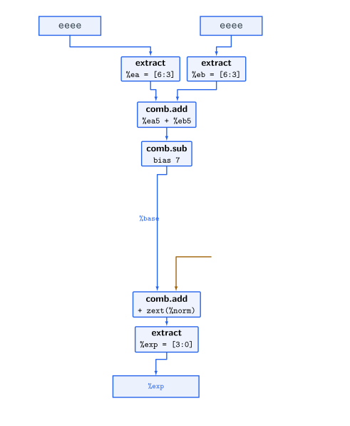
The blue box receives the two stored exponents and the normalization bit. It must produce %exp : i4:

\[ E_r=E_a+E_b-7+\mathtt{\%norm} \]

Your step: extract %ea and %eb, compute the expression above with five-bit intermediates, then extract the low four bits as %exp.

Exercise 7C: solution

E4M3 multiplier before exponent adjustment

\[ E_{\text{base}}=E_a+E_b-7, \qquad E_r=E_{\text{base}}+\mathtt{\%norm} \]

%norm is the bit computed in the previous stage: it is 1 exactly when the significand product was shifted right by one. Use five-bit intermediates to preserve the carry.

Exponent path

ea = comb.ExtractOp.create(3, i4, lhs).result
eb = comb.ExtractOp.create(3, i4, rhs).result
zero1 = hw.ConstantOp.create(i1, 0).result
ea5 = comb.ConcatOp.create(zero1, ea).result
eb5 = comb.ConcatOp.create(zero1, eb).result

sum_ = comb.AddOp.create(ea5, eb5).result
bias = hw.ConstantOp.create(i5, 7).result
base = comb.SubOp.create(sum_, bias).result
norm5 = comb.ConcatOp.create(zero4, norm).result
adjusted = comb.AddOp.create(base, norm5).result
exp = comb.ExtractOp.create(0, i4, adjusted).result

Solution checkpoint: exponent

Cumulative schematic

E4M3 multiplier with its exponent path completed

def lower_e4m3_mul(out_cast, rewriter):
    matched = match_e4m3_island(out_cast)
    if matched is None:
        return True
    lhs, rhs = matched
    with rewriter.ip:
        sa = comb.ExtractOp.create(7, i1, lhs).result
        sb = comb.ExtractOp.create(7, i1, rhs).result
        sign = comb.XorOp.create(sa, sb).result
        fa = comb.ExtractOp.create(0, i3, lhs).result
        fb = comb.ExtractOp.create(0, i3, rhs).result
        one = hw.ConstantOp.create(i1, 1).result
        ma4 = comb.ConcatOp.create(one, fa).result
        mb4 = comb.ConcatOp.create(one, fb).result
        zero4 = hw.ConstantOp.create(i4, 0).result
        ma8 = comb.ConcatOp.create(zero4, ma4).result
        mb8 = comb.ConcatOp.create(zero4, mb4).result
        product = comb.MulOp.create(ma8, mb8).result
        norm = comb.ExtractOp.create(7, i1, product).result
        direct = comb.ExtractOp.create(3, i4, product).result
        shifted = comb.ExtractOp.create(4, i4, product).result
        mant = comb.MuxOp.create(
            norm.value, shifted.value, direct.value).result
        frac = comb.ExtractOp.create(0, i3, mant).result
        ea = comb.ExtractOp.create(3, i4, lhs).result
        eb = comb.ExtractOp.create(3, i4, rhs).result
        zero1 = hw.ConstantOp.create(i1, 0).result
        ea5 = comb.ConcatOp.create(zero1, ea).result
        eb5 = comb.ConcatOp.create(zero1, eb).result
        sum_ = comb.AddOp.create(ea5, eb5).result
        bias = hw.ConstantOp.create(i5, 7).result
        base = comb.SubOp.create(sum_, bias).result
        norm5 = comb.ConcatOp.create(zero4, norm).result
        adjusted = comb.AddOp.create(base, norm5).result
        exp = comb.ExtractOp.create(0, i4, adjusted).result
        result = comb.ConcatOp.create(sign, exp, frac).result
    rewriter.replace_op(out_cast, [result])
    return False

Together: pack and replace

Complete normal-path E4M3 multiplier

Finally: pack the result.

The final value has the same i8 type as the output bitcast being replaced.

\[R=\{s,e,f\}\qquad\text{(Verilog notation)}\]

Finish the callback

result = comb.ConcatOp.create(sign, exp, frac).result
rewriter.replace_op(out_cast, [result])
return False

The floating-point island is dead; the greedy rewrite removes it.

Exercise 7: the simplified datapath

Cumulative schematic

Simplified E4M3 multiplier datapath

def lower_e4m3_mul(out_cast, rewriter):
    matched = match_e4m3_island(out_cast)
    if matched is None:
        return True
    lhs, rhs = matched
    with rewriter.ip:
        sa = comb.ExtractOp.create(7, i1, lhs).result
        sb = comb.ExtractOp.create(7, i1, rhs).result
        sign = comb.XorOp.create(sa, sb).result
        fa = comb.ExtractOp.create(0, i3, lhs).result
        fb = comb.ExtractOp.create(0, i3, rhs).result
        one = hw.ConstantOp.create(i1, 1).result
        ma4 = comb.ConcatOp.create(one, fa).result
        mb4 = comb.ConcatOp.create(one, fb).result
        zero4 = hw.ConstantOp.create(i4, 0).result
        ma8 = comb.ConcatOp.create(zero4, ma4).result
        mb8 = comb.ConcatOp.create(zero4, mb4).result
        product = comb.MulOp.create(ma8, mb8).result
        norm = comb.ExtractOp.create(7, i1, product).result
        direct = comb.ExtractOp.create(3, i4, product).result
        shifted = comb.ExtractOp.create(4, i4, product).result
        mant = comb.MuxOp.create(
            norm.value, shifted.value, direct.value).result
        frac = comb.ExtractOp.create(0, i3, mant).result
        ea = comb.ExtractOp.create(3, i4, lhs).result
        eb = comb.ExtractOp.create(3, i4, rhs).result
        zero1 = hw.ConstantOp.create(i1, 0).result
        ea5 = comb.ConcatOp.create(zero1, ea).result
        eb5 = comb.ConcatOp.create(zero1, eb).result
        sum_ = comb.AddOp.create(ea5, eb5).result
        bias = hw.ConstantOp.create(i5, 7).result
        base = comb.SubOp.create(sum_, bias).result
        norm5 = comb.ConcatOp.create(zero4, norm).result
        adjusted = comb.AddOp.create(base, norm5).result
        exp = comb.ExtractOp.create(0, i4, adjusted).result
        result = comb.ConcatOp.create(sign, exp, frac).result
    rewriter.replace_op(out_cast, [result])
    return False
patterns.add(arith.BitcastOp, lower_e4m3_mul)

Quiz: how many exact products did we prove?

How many normal \(\times\) normal cases does our restricted checker validate?

./scripts/test-e4m3-all.py --pass --normal-path
PASS: all 11892 E4M3 products match MLIR

11,892 of 56,644 normal \(\times\) normal pairs

That is 21% of normal \(\times\) normal, or 18% of all 65,536 bit-pattern pairs.

These are the guaranteed exact cases; truncation may coincide with correct rounding elsewhere.

Why does the checker stop at 11,892?

Outcome for normal \(\times\) normal Pairs
normal finite result 42,084
\(\hookrightarrow\) exact, no rounding 11,892
\(\hookrightarrow\) rounding required 30,192
subnormal result 3,916
underflow to zero 524
overflow to E4M3FN NaN 10,120
total 56,644

Our datapath still lacks:

  • round-to-nearest, ties-to-even;
  • subnormal and gradual-underflow paths;
  • exponent-range and overflow handling;
  • classification of zero, subnormal, and NaN inputs.

The 11,892 cases are exactly those for which none of this extra machinery is needed.

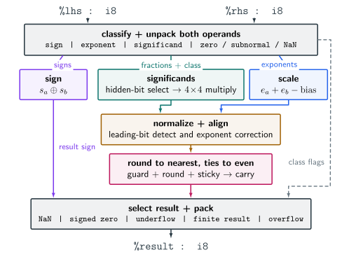
A complete E4M3FN multiplier

Block-level complete E4M3FN multiplier with classification, significand multiplication, scale computation, normalization, rounding, and special-case selection

A complete reference is provided, but we will not implement it today.

It handles:

  • operand and special-value classification;
  • normal/subnormal alignment and rounding;
  • zero, NaN, underflow, and overflow selection.
./scripts/test-e4m3-all.py
PASS: 65536 / 65536 products

Complete RTL is provided in exercises/.

And we are developing a tool

HAriCo can now generate an IEEE-754 single-precision adder directly as CIRCT Core IR:

$ ./build-circt/harico-cli --hdl circt IEEEFPAdd --wE 8 --wF 23
Info: CirctCodeGenerator.cpp: Now writing CIRCT Core IR to: harico.mlir

cat harico.mlir

module {
  hw.module @IEEEFPAdd_0_8_23_comb_uid21(
      in %X : i32, in %Y : i32, out R : i32) {
    %expX = comb.extract %X from 23 : (i32) -> i8
    %expY = comb.extract %Y from 23 : (i32) -> i8
    // ... exponent alignment, significand addition, normalization ...
  }
}

Generate hardware in hw + comb, then benefit from existing MLIR/CIRCT verification, optimization, and lowering passes.

From completeness to specialization

The complete reference expands numerical coverage.

We will instead exploit structure already visible in the IR.

Recognize %x * %x \(\longrightarrow\) generate a specialized squarer.

Exercise 8: should %x * %x cost the same?

Generic product

%p = arith.mulf %a, %b : f8E4M3FN

Square

%p = arith.mulf %x, %x : f8E4M3FN

What becomes simpler when both SSA operands are identical?

  1. \(s_x \oplus s_x = 0\): the normal finite result is positive.
  2. \(E_x + E_x = 2E_x\): one exponent is decoded and doubled.
  3. The significand partial-product matrix is symmetric.

The product matrix contains repeated work
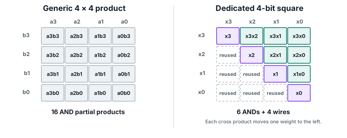
Comparison of the sixteen partial products in a generic four-bit multiplier with the six unique cross products and four diagonal wires in a four-bit squarer

For a square, the lower triangle duplicates the upper triangle and the diagonal does not require an AND gate (Dinechin and Kumm 2024, sec. 14.2).

Exercise 8: recognize the stronger pattern

cat exercises/ex8_e4m3fn_square.mlir
func.func @e4m3fn_square(%x : i8) -> i8 {
  %xf = arith.bitcast %x : i8 to f8E4M3FN
  %p = arith.mulf %xf, %xf : f8E4M3FN
  %r = arith.bitcast %p : f8E4M3FN to i8
  return %r : i8
}

Matcher excerpt: scripts/lower-e4m3fn-square.py

matched = match_e4m3_island(out_cast)
if matched is None:
    return True

lhs, rhs = matched
if lhs != rhs:
    return True

The rewrite continues only when both operands are the same SSA value. A combined production pass would give this pattern a higher PatternBenefit than the generic multiplier.

Exercise 8: build the 4-bit squarer - 12 min

Edit only: build_square4 in scripts/lower-e4m3fn-square.py.

def build_square4(value):
    i4 = IntegerType.get_signless(4)
    zero4 = hw.ConstantOp.create(i4, 0).result
    wide = comb.ConcatOp.create(zero4, value).result
    return comb.MulOp.create(wide, wide).result

This generic multiplier is the code to replace.

Task: return the exact 8-bit square of the 4-bit 1.mmm significand.

  • Route the four diagonal bits to weights \(2i\).
  • Compute the six distinct cross terms once and place them at \(i+j+1\).
  • Add the ten weighted terms into one i8 result.
  • Generate no comb.mul.

Everything outside this helper remains unchanged.

Exercise 8: generate and inspect

When your helper is ready:

python scripts/lower-e4m3fn-square.py \
  exercises/ex8_e4m3fn_square.mlir | \
  circt-tutorial-opt --tutorial-func-to-hw \
    --canonicalize \
    -o exercises/ex8_square_specialized.mlir
grep -n "comb.mul" exercises/ex8_square_specialized.mlir  # no match

The generated file must be created, pass MLIR verification, and contain no comb.mul. Functional equivalence and circuit cost are checked after the solution.

Solution checkpoint: diagonal terms

For every bit \(x_i\):

\[x_i^2=x_i\]

Its weight changes from \(i\) to \(2i\). Extending one bit to i8 and shifting it by a constant describes that wiring.

At this checkpoint, terms contains only the four diagonal wires.

def build_square4(value):
    i1 = IntegerType.get_signless(1)
    i7 = IntegerType.get_signless(7)
    i8 = IntegerType.get_signless(8)
    bits = [
        comb.ExtractOp.create(i, i1, value).result
        for i in range(4)
    ]
    zero7 = hw.ConstantOp.create(i7, 0).result

    def at_weight(bit, weight):
        wide = comb.ConcatOp.create(zero7, bit).result
        shift = hw.ConstantOp.create(i8, weight).result
        return comb.ShlOp.create(wide, shift).result

    terms = [at_weight(bits[i], 2 * i) for i in range(4)]

Solution checkpoint: cross terms

For each pair \(j<i\):

\[2x_ix_j=x_ix_j\,2^1\]

Compute one AND and place it at weight \(i+j+1\). The nested loop visits the six distinct cross terms; comb.add collects all ten weighted terms.

def build_square4(value):
    i1 = IntegerType.get_signless(1)
    i7 = IntegerType.get_signless(7)
    i8 = IntegerType.get_signless(8)
    bits = [
        comb.ExtractOp.create(i, i1, value).result
        for i in range(4)
    ]
    zero7 = hw.ConstantOp.create(i7, 0).result
    def at_weight(bit, weight):
        wide = comb.ConcatOp.create(zero7, bit).result
        shift = hw.ConstantOp.create(i8, weight).result
        return comb.ShlOp.create(wide, shift).result
    terms = [at_weight(bits[i], 2 * i) for i in range(4)]
    for i in range(4):
        for j in range(i):
            cross = comb.AndOp.create(bits[i], bits[j]).result
            terms.append(at_weight(cross, i + j + 1))
    return comb.AddOp.create(*terms).result

Exercise 8: prove, then measure

Generate the generic Exercise 7 baseline:

python solutions/lower-e4m3fn-normal.py \
  exercises/ex8_e4m3fn_square.mlir | \
  circt-tutorial-opt --tutorial-func-to-hw \
    --canonicalize -o exercises/ex8_square_generic.mlir

Compare it with the specialized circuit:

./scripts/compare-aig.py \
  exercises/ex8_square_generic.mlir \
  exercises/ex8_square_specialized.mlir \
  e4m3fn_square
Lowering checkpoint AIG nodes Levels
generic Exercise 7 multiplier 57 14
supplied square intermediate 51 14
dedicated significand squarer 50 13

Match more intent; build better datapaths

The same rewrite strategy extends beyond one squarer:

Recognized arithmetic Possible datapath
%x * %x dedicated squarer
%x * C constant multiplier or shift-add network
%a * %b + %c fused multiply-add with one final rounding
\(\sum_i x_i^2\) fused sum-of-squares datapath
dot product or polynomial target-sized fused operator

MLIR preserves enough intent to recognize the pattern; CIRCT lets the pass materialize the chosen circuit. This is the bridge to higher-level hardware generation.

Conclusion

Compilation becomes hardware design…

or the other way around?

What we did

  • Started from the motivation: the end of free scaling and the power, memory, and communication walls demand specialization all the way down to hardware — calling for compiler techniques that help design the machine.

  • Practised digital design with CIRCT: represented hierarchy, combinational logic, and state; then transformed, verified, synthesized, and emitted the design.

  • Built an application-specific circuit: lowered arith.mulf to an E4M3 comb datapath, then recognized %x * %x to generate a cheaper squarer.

Yes: we can do digital design with MLIR and CIRCT — and it is interesting!

Where I want to take this

My research asks how to connect a complete HLS flow to an automated design-space exploration loop:

  • Full HLS flow: lower tensor / linalg through scheduling, memory, control, and arithmetic decisions into CIRCT, RTL, and physical implementation.

  • Design-space exploration (DSE): generate architectural variants, prove their behavior, compare accuracy, area, timing, and power, and feed those measurements back into the compiler.

Bonus: HLS with MLIR and CIRCT

Progressive Arithmetic Lowering from Tensor Kernels to Synthesizable Datapaths

Inria

INSA Lyon

CITI Lab

ANR

Louis Ledoux
Pierre Cochard
Florent de Dinechin

Progressive Arithmetic Lowering from Tensor Kernels to Synthesizable Datapaths

MLIR Workshop @ Euro LLVM Developers’ Meeting
13 April 2026

Motivation: AI

class LlamaFfnSublayer(nn.Module):
    """Llama FFN sublayer using SwiGLU."""

    def __init__(
        self,
        dim: int = 512,
        hidden_dim: int | None = None,
        multiple_of: int = 256,
    ):
        super().__init__()
        if hidden_dim is None:
            hidden_dim = 4 * dim
            hidden_dim = int(2 * hidden_dim / 3)
            hidden_dim = multiple_of * (
                (hidden_dim + multiple_of - 1)
            )
        self.w_gate = nn.Linear(dim, hidden_dim, bias=False)
        self.w_up = nn.Linear(dim, hidden_dim, bias=False)
        self.w_down = nn.Linear(hidden_dim, dim, bias=False)

    def forward(self, x: torch.Tensor) -> torch.Tensor:
        gate = F.silu(self.w_gate(x))
        up = self.w_up(x)
        return self.w_down(gate * up)
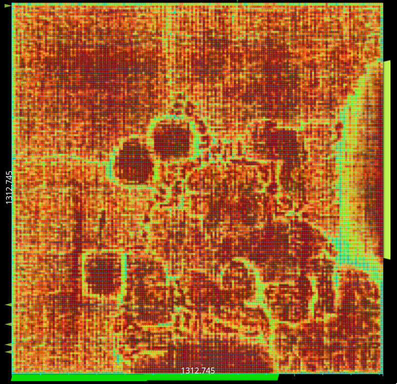
Llama ASIC routing congestion heat map

Llama ASIC routing

Motivation: Audio DSP
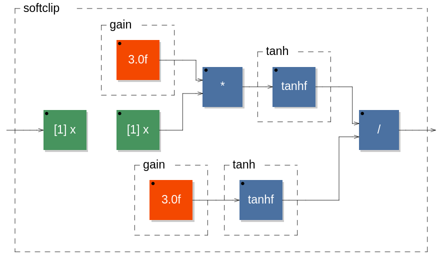
// Soft clipping waveshaper.
// Hyperbolic tangent via foreign function.

gain = 3.0;

tanh = ffunction(float tanhf|tanh|tanhl (float), <math.h>, "");

softclip(x) = tanh(gain * x) / tanh(gain);

process = _,_ : par(i, 2, softclip);

Soft-clipping signal-flow graph

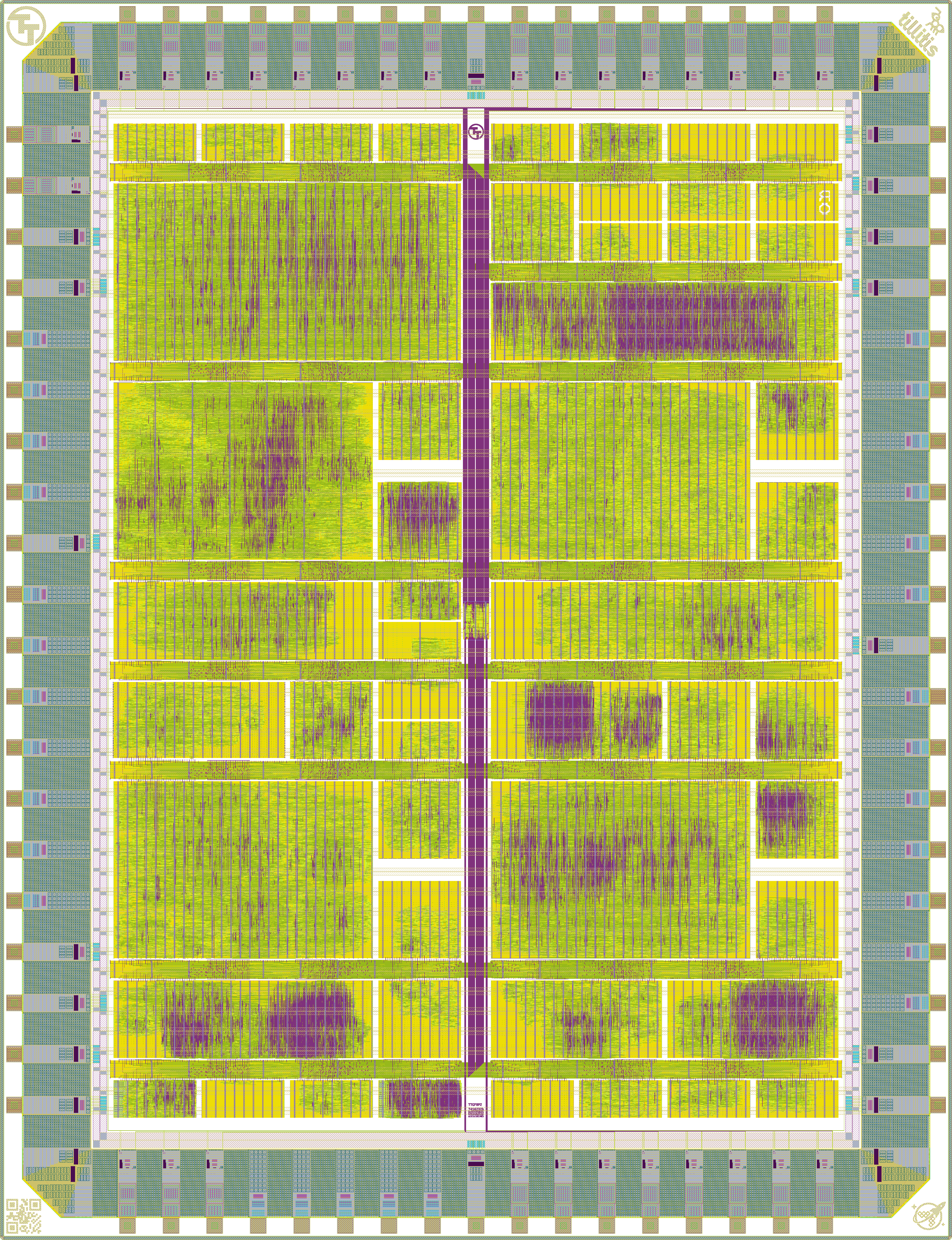
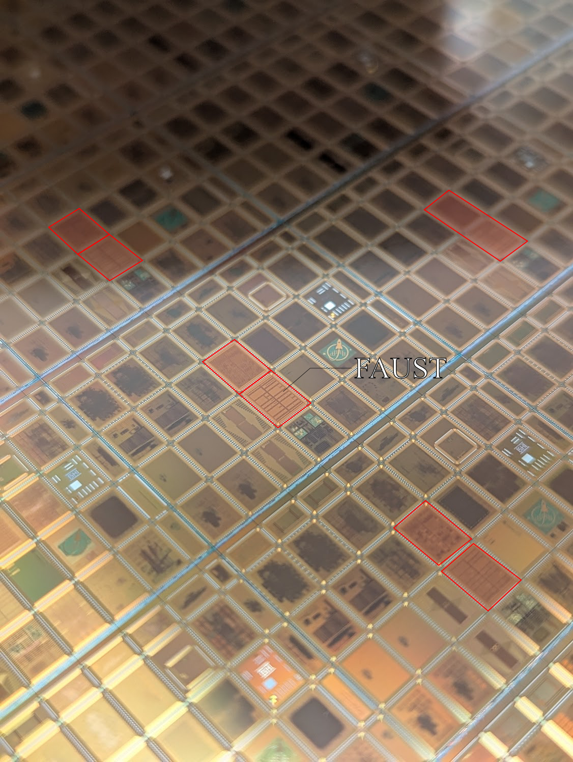
TinyTapeout GF0P02 wafer Annotated TinyTapeout GF0P02 wafer

TinyTapeout GF0P02 wafer.space

Problem to silicon crosses many intermediate arithmetic levels.

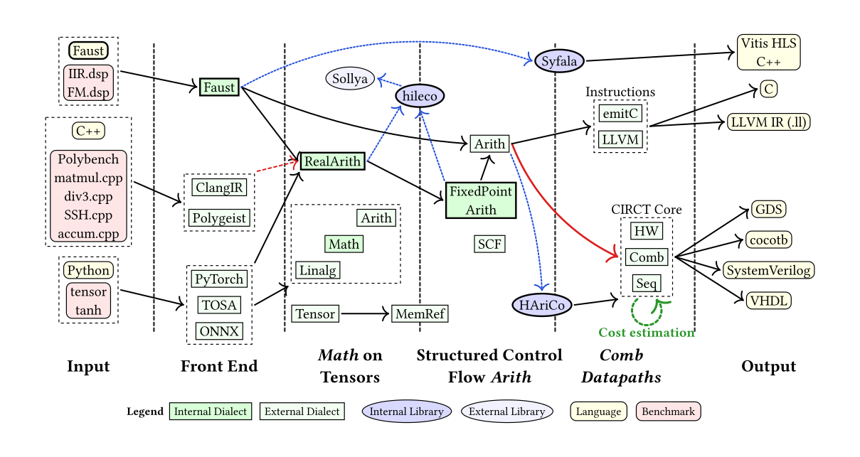
Emeraude-MLIR

Our take on the end-to-end levels
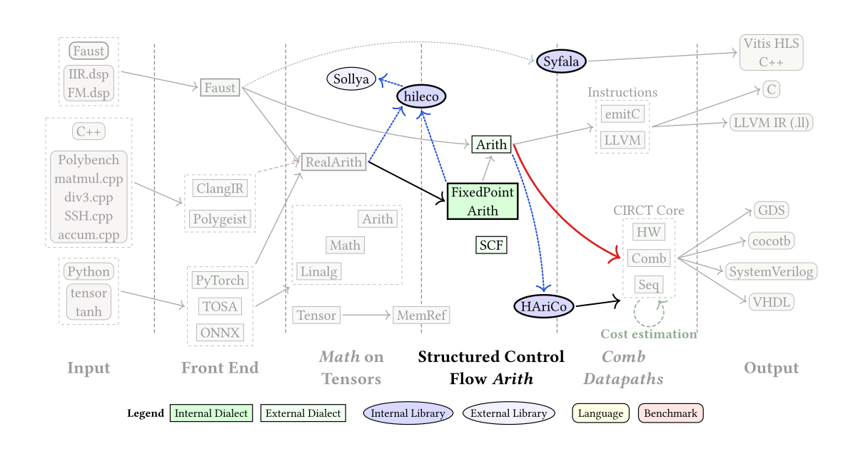
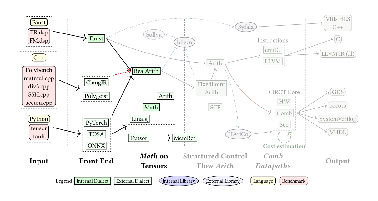
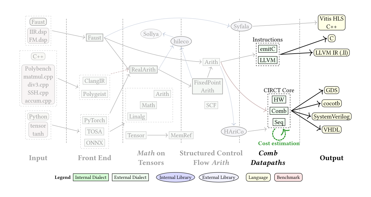
Complete Emeraude-MLIR compilation levels Front-end and high-level arithmetic focus Structured control flow and arithmetic focus Datapath and output focus

Motivations at both ends: frontends and backends

Frontends on one hand

Faust / DSP
  • FIR / IIR recurrences on sample streams
  • Fixed-point friendly audio kernels
  • Nonlinear audio functions: saturation, waveshaping, modal/finite-difference-time-domain physical modelling
  • Precision control: range, quantization, overflow
Tensor / ML
  • Tensor contractions: (matmul, batched GEMM)
  • Nonlinear kernels: SiLU / exp / sigmoid / softmax
  • Accumulation depth: rounding-error growth
  • Precision control: mixed-precision per layer

Arithmetic motivations of different natures

Backends on the other hand

PPA objectives: area, power, performance…
… or budgets / constraints

FPGA
  • Resource budgets: LUT, FF, BRAM, DSP
  • Reconfigurable
  • Throughput-oriented
ASIC
  • Standard cells (Resizing)
  • Process Design Kit
    • 7nm, 180nm, corners, high density
  • Physical constraints: congestion, wiring
  • DRC/LVS and signoff requirements

Hardware constraints of different natures

High-level math on tensors

Polynomial approximations

  • RealArith and FixedPointArith.
  • --realarith-to-fixed_pt_arith for polynomial approximation lowering.
  • Horner Scheme

Two degree-16 polynomial approximations

2 × degree-16

Thirty-two degree-4 polynomial approximations

32 × degree-4

Example 1: \(f(x)=\tanh(3x)/\tanh(3)\)

--realarith-to-fixed_pt_arith="approximation-method=uniform_piecewise_poly polynomial-degree=10 coeff-storage=switch"

index_switch: 8 intervals (cases 0..7)

P0(h) = ((((((((((-78h + 46)h + 1454)h + -7314)h + -78970)h + 682179)h +
4256867)h + -57922167)h + -191490613)h + 5510525043)h + 5640589127

\(\left[\ldots\right]\)

P7(h) = ((((((((((83h + -18)h + -206)h + 65)h + -477)h + 12014)h +
-170708)h + 1874477)h + -15214840)h + 81733304)h + 30216113779
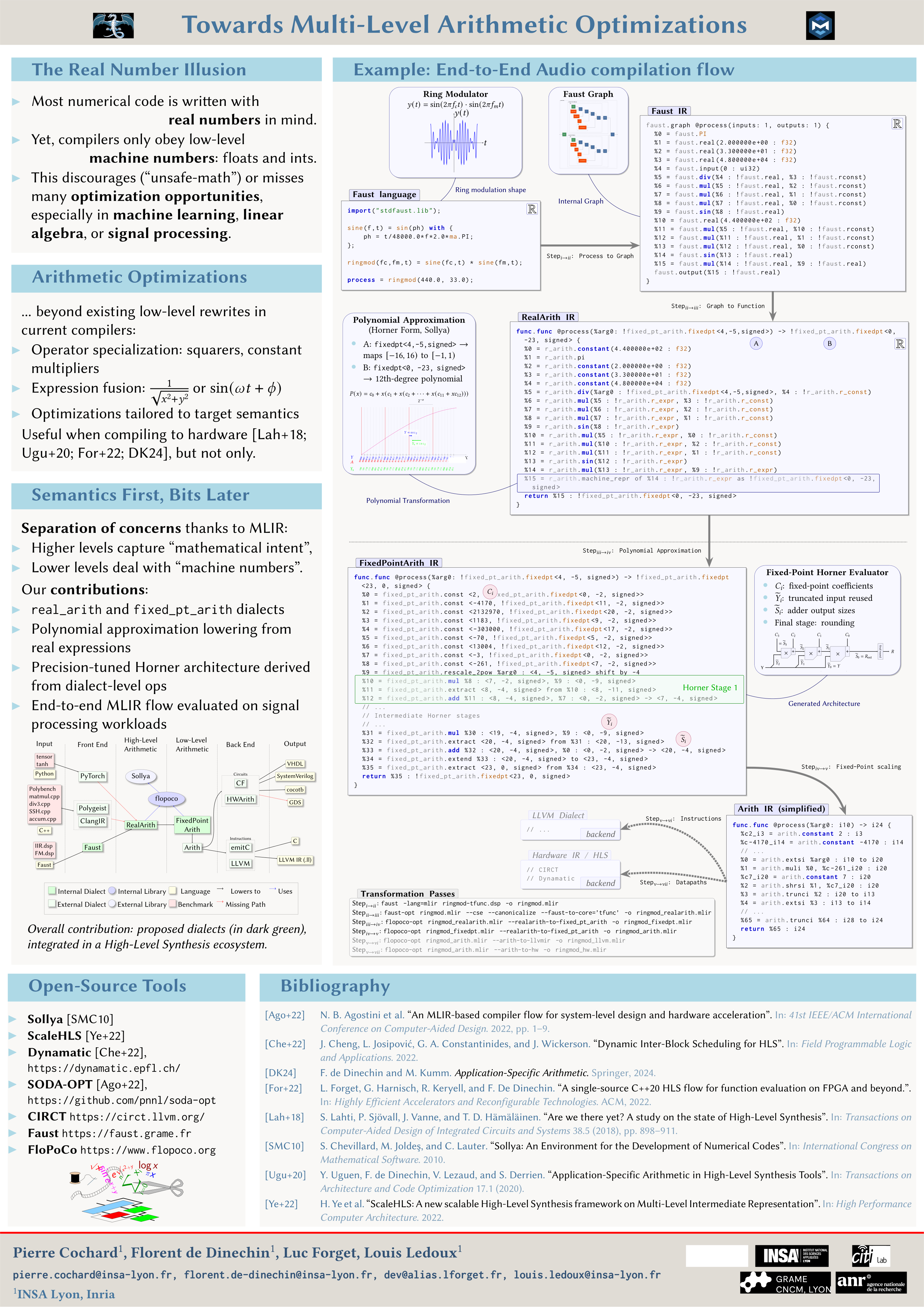
EuroLLVM 2025 poster

EuroLLVM 2025 poster
https://hal.science/hal-05063466

Example on an LLM subkernel
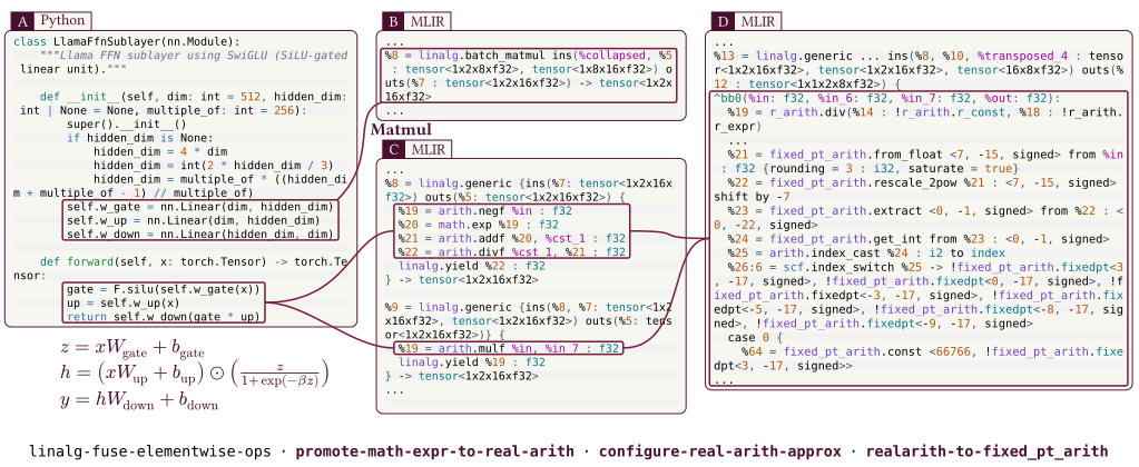
Annotated Python and MLIR lowering for a Llama FFN subkernel

High-level optimization potential:
linear algebra kernels & nonlinear functions.

Medium-level arith on SCF and memrefs

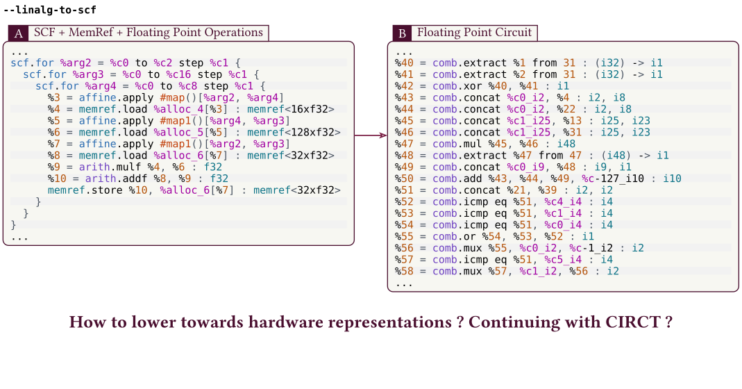
The gap from MLIR to CIRCT

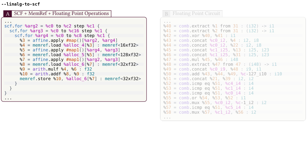
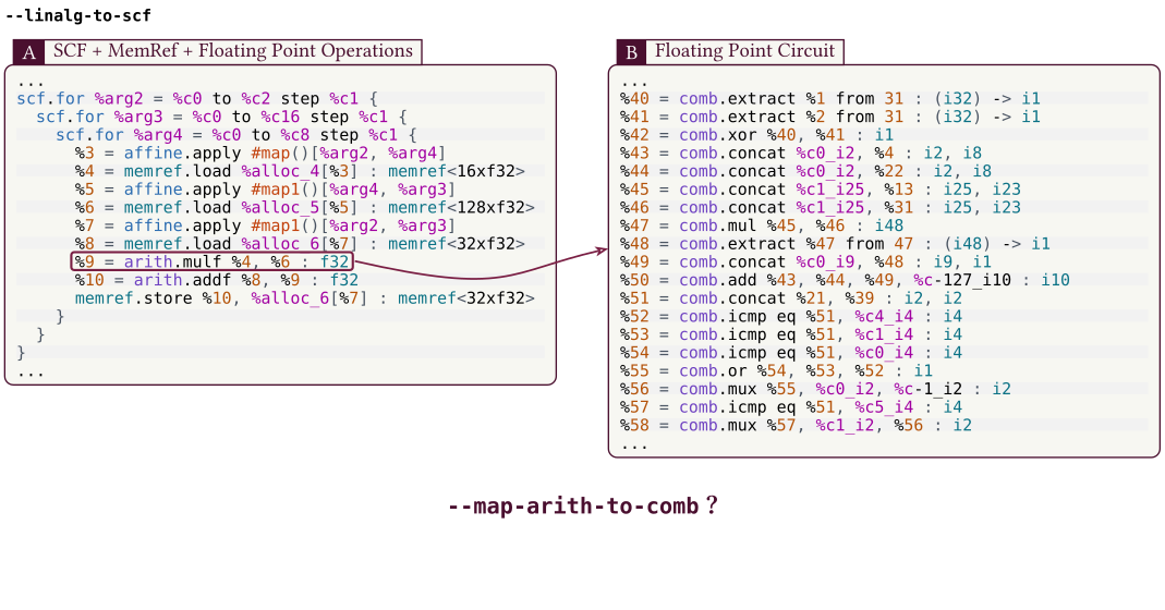
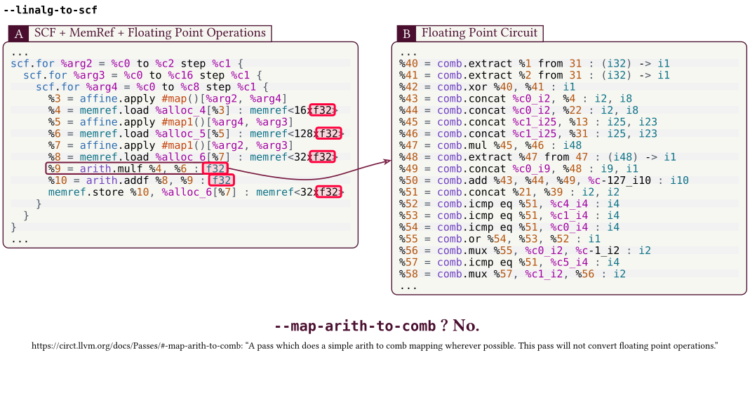
SCF floating-point accumulation before CIRCT lowering Question about lowering SCF floating-point operations to hardware Attempt to use map-arith-to-comb for floating-point operations Map-arith-to-comb rejection with every f32 type highlighted

Approaches in the literature

Representative approaches
  • ScaleHLS / StreamTensor [1][2]
  • Dynamatic [3]
  • BASE2 [4]
Common limitation

Final floating-point implementation is delegated to vendor HLS or IP/core generators.

AMD/Xilinx documentation

“float and double … are synthesized with IEEE-754 standard partial compliance.”

“complies with much of the IEEE-754 Standard … deviations generally provide a better trade-off of resources.”

[1] Ye et al., HPCA 2022 · [2] Ye & Chen, MICRO 2025 · [3] Xu et al., FPGA 2023 · [4] Friebel et al., HEART 2023

Partial compliance + hidden vendor IP ⇒ opaque arithmetic behavior and limited control.

Low-level datapaths with comb, seq, and HW

Comb/seq and cost estimation

  • CIRCT Core: Comb/Seq/HW
  • Cost modeling
    • AIG, MIG, High-Level Heuristics
  • Avoid commiting to hardware
  • Native AIG export: circt-translate <synth.mlir> --export-aiger -o 90-final.aig
  • Fallback AIG export: hls-driver/scripts/export-aig-via-yosys-abc.sh <circt-opt> <in.mlir> 90-final.aig forward
  • PPA in seconds
  • Preparing QoR / DSE
module {
  hw.module @forward(in %arg0 : !hw.array<16xi32>, in %arg1 : !hw.array<16xi32>, in %clk : !seq.clock, in %reset : i1, out arg1_out : !hw.array<16xi32>) {
    ...
    %111 = comb.extract %local_mem_2_rdata from 31 : (i32) -> i1
    %112 = comb.extract %local_mem_3_rdata from 31 : (i32) -> i1
    %113 = comb.xor %111, %112 : i1
    %114 = comb.extract %local_mem_2_rdata from 23 : (i32) -> i8
    %115 = comb.extract %local_mem_3_rdata from 23 : (i32) -> i8
    %118 = comb.concat %c1_i25, %116 : i25, i23
    %120 = comb.mul %118, %119 : i48
    %123 = comb.add %114, %115, %122, %c-127_i8 : i8
    ...
  }
}
module forward(
  input  [15:0][31:0] arg0,
                      arg1,
  input               clk,
                      reset,
  output [15:0][31:0] arg1_out
);
  wire [511:0] _GEN_57 = arg0;
  reg  [31:0]  arg1_mem[0:15];
  always_ff @(posedge clk) begin
    if (!reset) begin
      if (_GEN_5) arg1_mem[_GEN_1] <= _GEN_0;
      if (_GEN_9) arg1_mem[_GEN_6] <= 32'h0;
    end
  end
  ...
endmodule

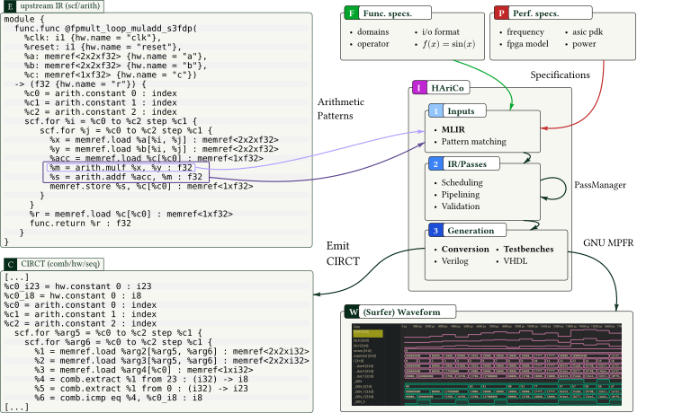
HAriCo

Introducing HAriCo (Hardware Arithmetic Cores)

  • IR-based FloPoCo implementation
    • Modernized C++ API
    • Multiple outputs
      • VHDL, SystemVerilog, MLIR, …
    • Conversion & transformation passes
  • C API (Python, Rust bindings)
  • Big code-base (approx. 90 operators)
    • (will take time…)

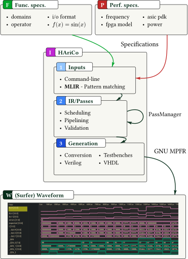
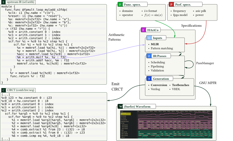
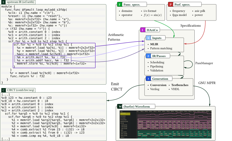
HAriCo architecture and waveform

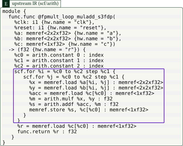
HAriCo input IR

SCF and arithmetic loop selected for hardware materialization

Three materialization strategies

1Per-op
  • IEEE754-compliant
  • 1 Operation → 1 Operator
  • N Operations → N Roundings
2Fused-graph-datapath
  • FMA philosophy
  • 1 deferred rounding
  • Expression fusion

\[ \frac{1}{\sqrt{x^2+y^2}} \qquad \sin(\omega t + \varphi) \]
3Specialized
  • Squarers [1]
  • Constant multipliers [2]
  • Kulisch / Systolic Arrays [3]
  • Target semantics

Systolic array architecture

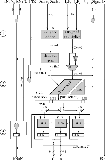
Specialized floating-point datapath

From MLIR to CIRCT: harico-arith-to-comb

1Per-op
  • IEEE754-compliant
  • 1 Operation → 1 Operator
  • N Operations → N Roundings

Per-operation pattern selected in the HAriCo lowering flow

1. emeraude-mlir-opt in.mlir --harico-arith-to-comb="lowering-mode=per-op target=VirtexUltraScale target-frequency=2.5e7"
2Fused-graph-datapath
  • FMA philosophy
  • 1 deferred rounding
  • Expression fusion

\[ \frac{1}{\sqrt{x^2+y^2}} \qquad \sin(\omega t + \varphi) \]

Fused-graph pattern selected in the HAriCo lowering flow

2. emeraude-mlir-opt in.mlir --harico-arith-to-comb="lowering-mode=fused-graph-datapath target=sky130 target-frequency=2.5e7"
3Specialized
  • Squarers
  • Constant multipliers
  • Kulisch / Systolic Arrays
  • Target semantics

Specialized floating-point datapath

Specialized loop pattern selected in the HAriCo lowering flow

3. emeraude-mlir-opt in.mlir --harico-arith-to-comb="lowering-mode=specialized specializations=enable=s3fdp,s3fdp.chunk_size=32,s3fdp.ovf=10,s3fdp.msb=10,s3fdp.lsb=-20 target=tsmc7 target-frequency=2.5e7"

HAriCo C++ API example

#include <HAriCo/Context.hpp>
#include <HAriCo/Operators/FPAddSinglePath.hpp>
using namespace HAriCo;

auto ctx = Context::new_default();
ctx.options["target"] = Targets::VirtexUltraScalePlus;
ctx.options["frequency"] = 500 // MHz;

// Build operator:
auto op = FPAdd();
auto options = op.interface(ctx);
options["wE"] = 8;
options["wF"] = 23;
Module mod = op.build(ctx, options);

// Before pass:
VerilogCodeGenerator gen;
gen.build(mod).fwrite("fpadd.sv");

PassManager pm;
pm.add<TimingAnalysisPass>();
pm.add<SchedulePass>();
pm.add<PipelineizePass>();
pm.run(mod);
gen.build(mod).fwrite("fpadd_pipeline.sv");

HAriCo Python bindings example

import harico as hrc

def main():
    ctx = hrc.Context()
    ctx.set_target("VirtexUltrascalePlus", frequency_mhz=500)

    op = hrc.Operator("FPAdd")
    mod = op.build_ir(
        ctx,
        wE=8,
        wF=23,
        sub=False,
        dualPath=False,
        onlyPositiveIO=False,
    )

    # Before pass:
    mod.emit_vhdl("fpadd_before_pipelineize.vhd")
    mod.emit_verilog("fpadd_before_pipelineize.v")

    # Analysis passes first:
    pm_analysis = hrc.PassManager(["timing", "schedule"])
    pm_analysis.run(mod, ctx)

    # Transform pass:
    pm_pipelineize = hrc.PassManager(["pipelineize"])
    pm_pipelineize.run(mod, ctx)

Results: DSP

Wafer.space run

TinyTapeout wafer layout for the Faust design

MPW + TT submission (TTg0p2) on Wafer.space — Utilisation 47.106% · Wire length 377542 um

GDS 3D view
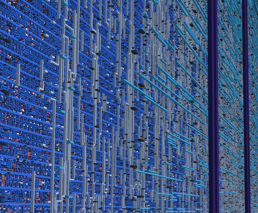
Three-dimensional GDS view

Reticle view (wafer.space)

Wafer.space reticle view

Results: LLM and HAriCo lowering strategies

ASIC: GDS routing congestion

ASIC SKY130HD Llama

Metric Value
Area 1.7233 mm²
Die Dimensions 1.312 × 1.312 mm
Power Breakdown
Combinational 0.117 W
Sequential 0.044 W
Clock 0.028 W
Total Power 0.189 W

Llama routing congestion heat map

Llama 1.5 mm² routing congestion heatmap

FPGA: resource usage

FPGA VU19P Llama

Metric Value
LUTs 26,928
Flip-Flops 12,221
DSP Blocks 17

Llama placement and routing on a VU19P FPGA

Llama FPGA vu19p P&R

Llama FFN sublayer

module {
  func.func @forward(%arg0: tensor<1x2x8xf32>) -> tensor<1x2x8xf32> {
    %7 = linalg.batch_matmul ... -> tensor<1x2x16xf32>
    %8 = linalg.generic ... ins(%7 : tensor<1x2x16xf32>) outs(%5 : tensor<1x2x16xf32>) {
    ^bb0(%in: f32, %out: f32):
      %neg = arith.negf %in : f32
      %exp = math.exp %neg : f32
      %gate = arith.divf %cst_1, %den : f32
      %silu = arith.mulf %in, %gate : f32
      linalg.yield %silu : f32
    } -> tensor<1x2x16xf32>
    return %18 : tensor<1x2x8xf32>
  }
}
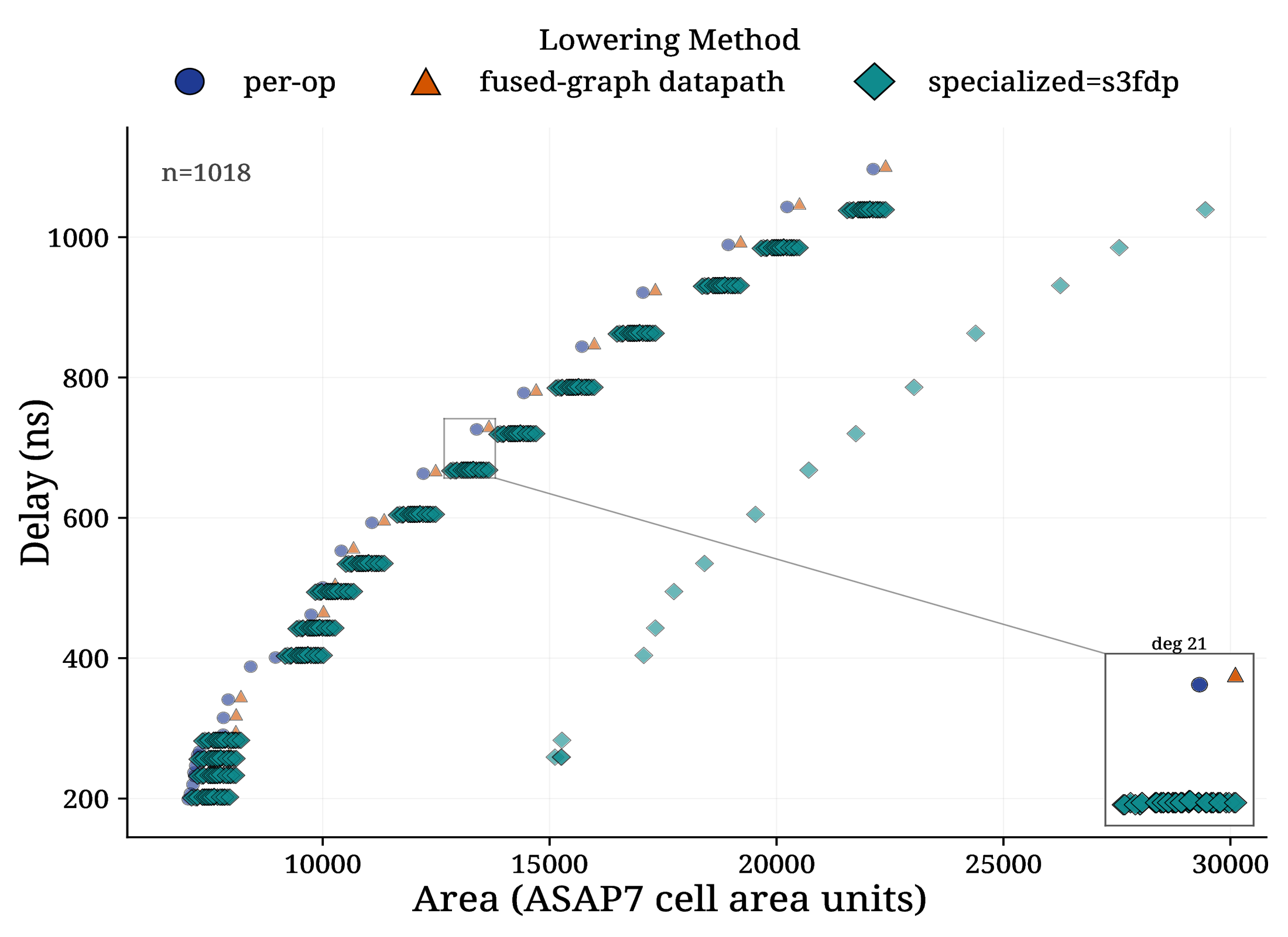
Llama FFN Sublayer area versus delay

Llama FFN Sublayer. Area vs. Delay

MatMul + SiLU

#map = affine_map<(d0, d1) -> (d0, d1)>
module {
  func.func @forward(%arg0: tensor<2x4xf32>) -> tensor<2x4xf32> {
    %mm = linalg.matmul ... -> tensor<2x4xf32>
    %sig = linalg.generic ... ins(%mm : tensor<2x4xf32>) outs(%empty : tensor<2x4xf32>) {
    ^bb0(%in: f32, %acc: f32):
      %neg = arith.negf %in : f32
      %exp = math.exp %neg : f32
      %gate = arith.divf %c1, %den : f32
      linalg.yield %gate : f32
    } -> tensor<2x4xf32>
    %out = linalg.generic ... ins(%sig, %mm : tensor<2x4xf32>, tensor<2x4xf32>) outs(%empty : tensor<2x4xf32>)
    return %out : tensor<2x4xf32>
  }
}
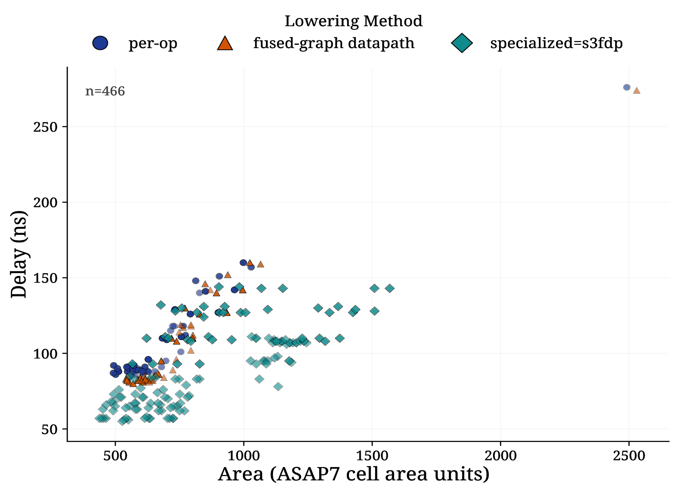
MatMul plus SiLU area versus delay

MatMul + SiLU. Area vs. Delay

MatMul + sigmoid

#map = affine_map<(d0, d1) -> (d0, d1)>
module {
  func.func @forward(%arg0: tensor<2x4xf32>) -> tensor<2x4xf32> {
    %mm = linalg.matmul ... -> tensor<2x4xf32>
    %out = linalg.generic ... ins(%mm : tensor<2x4xf32>) outs(%empty : tensor<2x4xf32>) {
    ^bb0(%in: f32, %acc: f32):
      %neg = arith.negf %in : f32
      %exp = math.exp %neg : f32
      %sig = arith.divf %c1, %den : f32
      linalg.yield %sig : f32
    } -> tensor<2x4xf32>
    return %out : tensor<2x4xf32>
  }
}
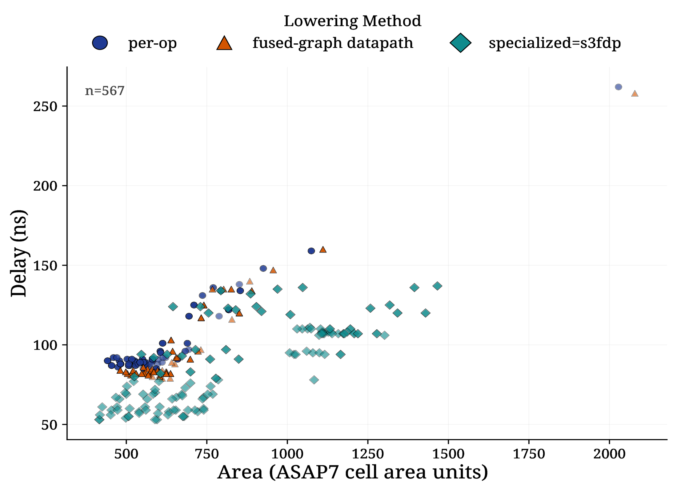
MatMul plus sigmoid area versus delay

MatMul + Sigmoid. Area vs. Delay

Attention softmax exponential

#map = affine_map<(d0, d1) -> (d0, d1)>
module {
  func.func @forward(%query: tensor<2x4xf32>) -> tensor<2x2xf32> {
    %score = linalg.matmul ... -> tensor<2x2xf32>
    %out = linalg.generic ... ins(%score : tensor<2x2xf32>) outs(%out_empty : tensor<2x2xf32>) {
    ^bb0(%in: f32, %acc: f32):
      %res = math.exp %in : f32
      linalg.yield %res : f32
    } -> tensor<2x2xf32>
    return %out : tensor<2x2xf32>
  }
}
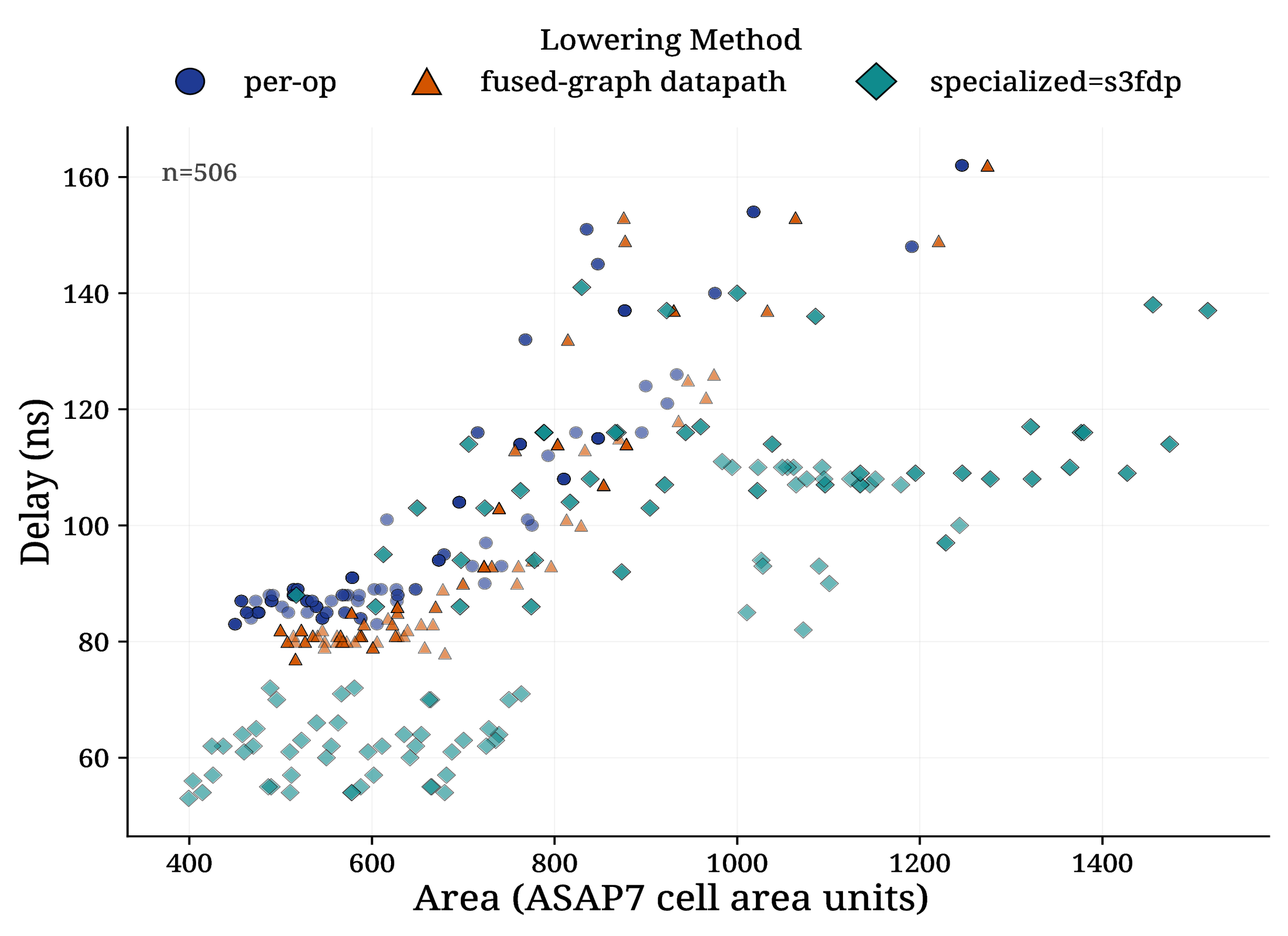
Attention softmax exponential area versus delay

Attention Softmax Exponential. Area vs. Delay

MatMul + sigmoid heavy-tail

#map = affine_map<(d0, d1) -> (d0, d1)>
module {
  func.func @forward(%arg0: tensor<2x8xf32>) -> tensor<2x8xf32> {
    %mm = linalg.matmul ... -> tensor<2x8xf32>
    %out = linalg.generic ... ins(%mm : tensor<2x8xf32>) outs(%empty : tensor<2x8xf32>) {
    ^bb0(%in: f32, %acc: f32):
      %neg = arith.negf %in : f32
      %exp = math.exp %neg : f32
      %res = arith.divf %c1, %den : f32
      linalg.yield %res : f32
    } -> tensor<2x8xf32>
    return %out : tensor<2x8xf32>
  }
}
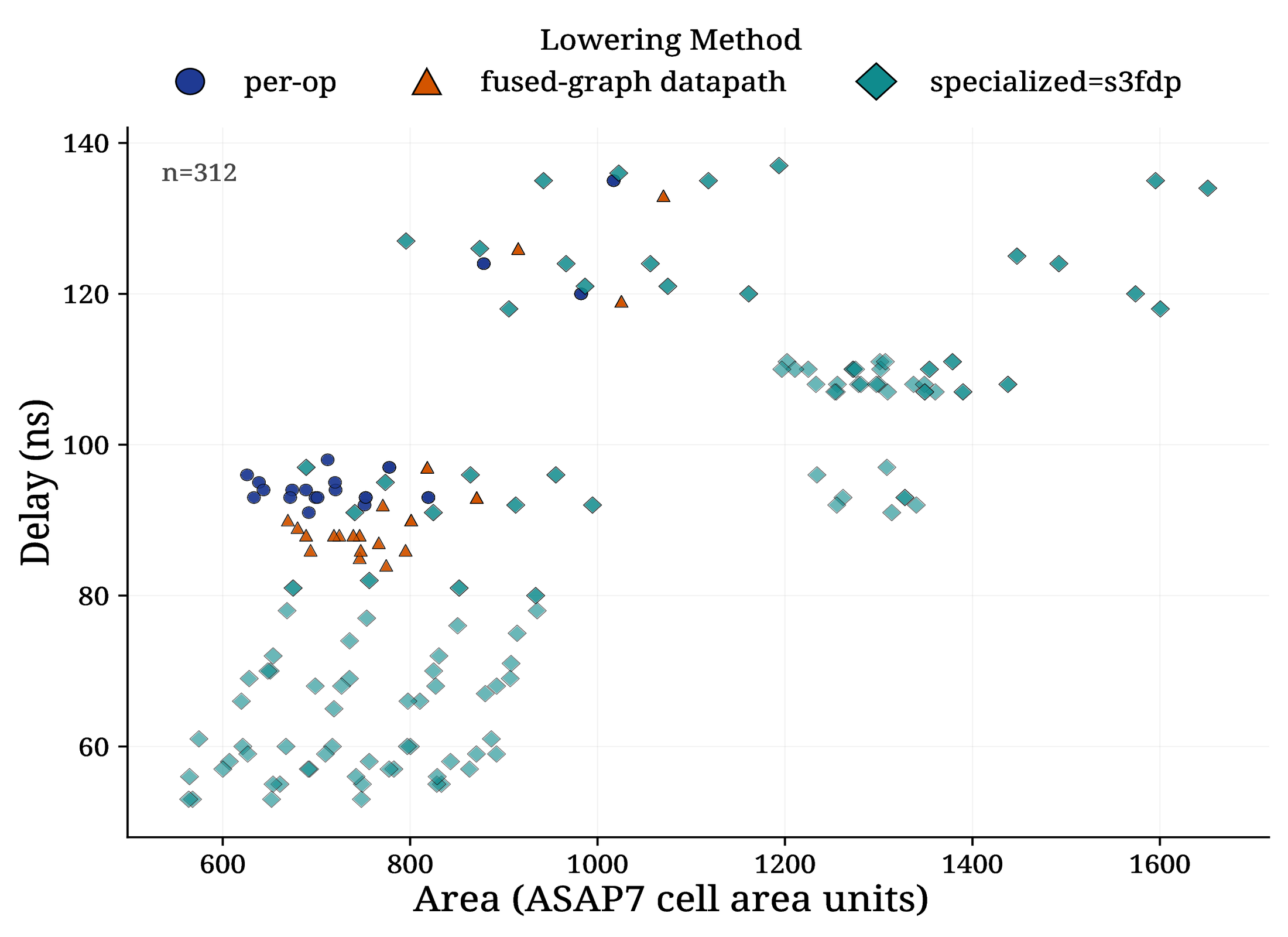
MatMul plus sigmoid heavy-tail area versus delay

MatMul + Sigmoid Heavy-Tail. Area vs. Delay

GEMV accumulation

module {
  func.func @forward(%arg0: tensor<1x4xf32>) -> tensor<1x4xf32> {
    %w = arith.constant dense<...> : tensor<4x4xf32>
    %init = linalg.fill ins(%c0 : f32) outs(%empty : tensor<1x4xf32>) -> tensor<1x4xf32>
    %out = linalg.matmul ins(%arg0, %w : tensor<1x4xf32>, tensor<4x4xf32>) outs(%init : tensor<1x4xf32>)
      -> tensor<1x4xf32>
    return %out : tensor<1x4xf32>
  }
}
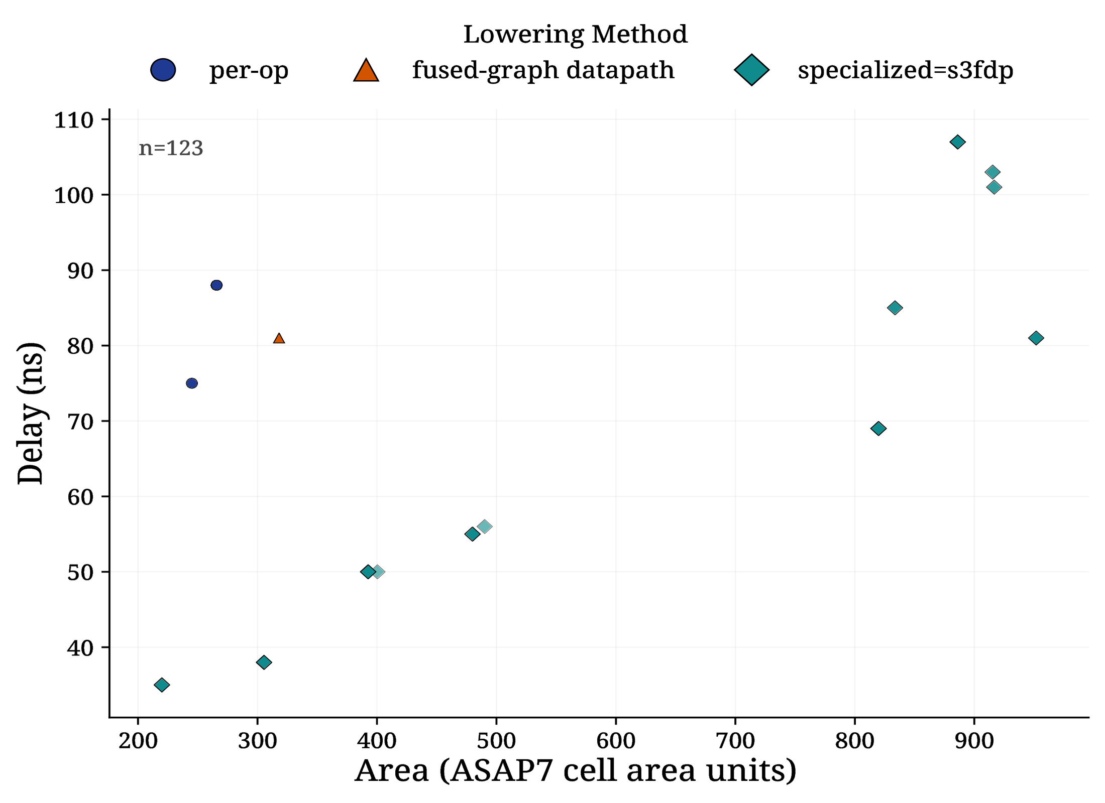
GEMV accumulation area versus delay

GEMV Accumulation. Area vs. Delay

Attention score

module {
  func.func @forward(%query: tensor<2x4xf32>) -> tensor<2x2xf32> {
    %kt = arith.constant dense<...> : tensor<4x2xf32>
    %init = linalg.fill ins(%c0 : f32) outs(%empty : tensor<2x2xf32>) -> tensor<2x2xf32>
    %score = linalg.matmul ins(%query, %kt : tensor<2x4xf32>, tensor<4x2xf32>) outs(%init : tensor<2x2xf32>)
      -> tensor<2x2xf32>
    return %score : tensor<2x2xf32>
  }
}
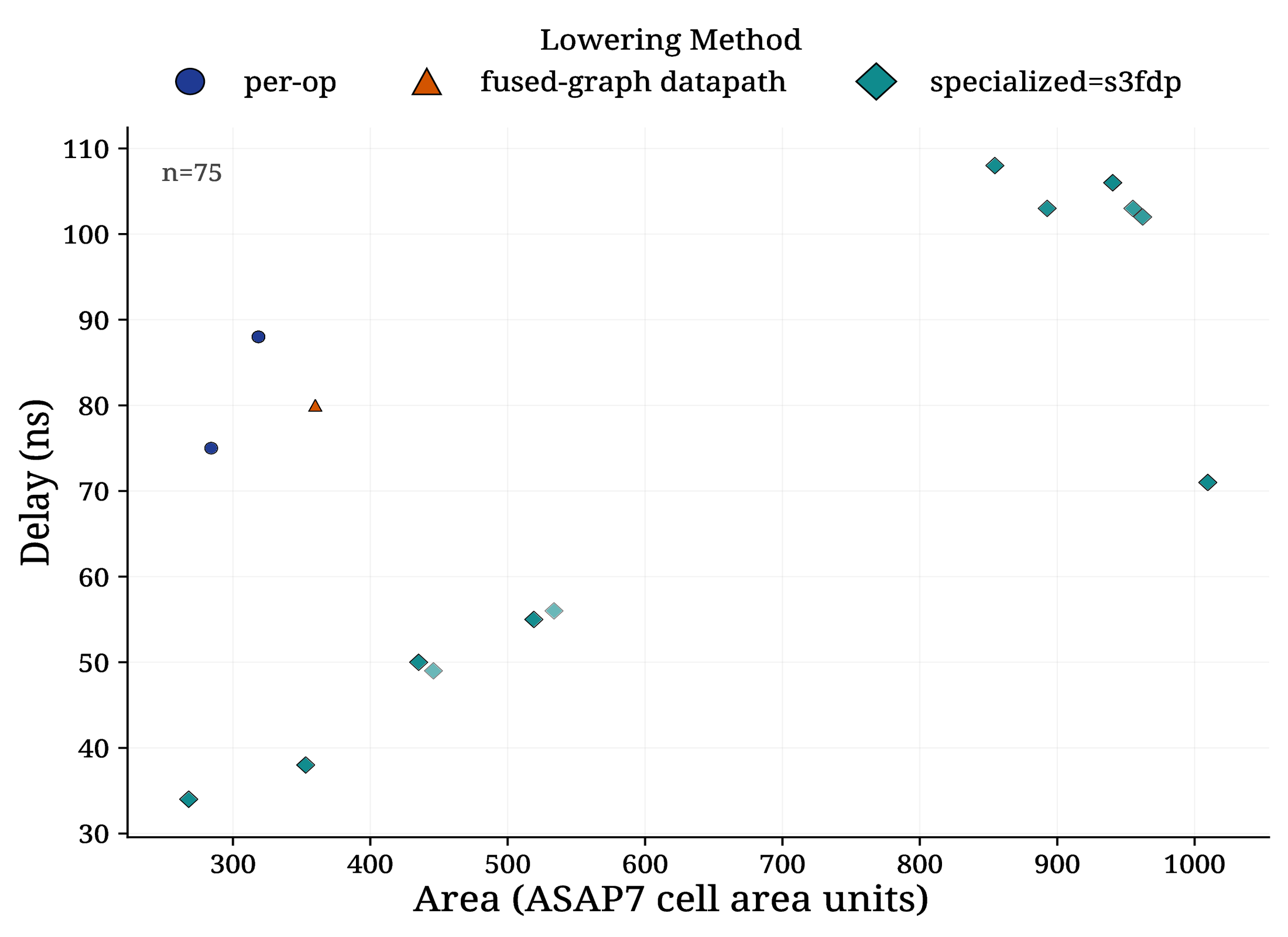
Attention score area versus delay

Attention Score. Area vs. Delay

MatMul accumulation

module {
  func.func @forward(%arg0: tensor<2x4xf32>) -> tensor<2x4xf32> {
    %w = arith.constant dense<...> : tensor<4x4xf32>
    %init = linalg.fill ins(%c0 : f32) outs(%empty : tensor<2x4xf32>) -> tensor<2x4xf32>
    %mm = linalg.matmul ins(%arg0, %w : tensor<2x4xf32>, tensor<4x4xf32>) outs(%init : tensor<2x4xf32>)
      -> tensor<2x4xf32>
    return %mm : tensor<2x4xf32>
  }
}
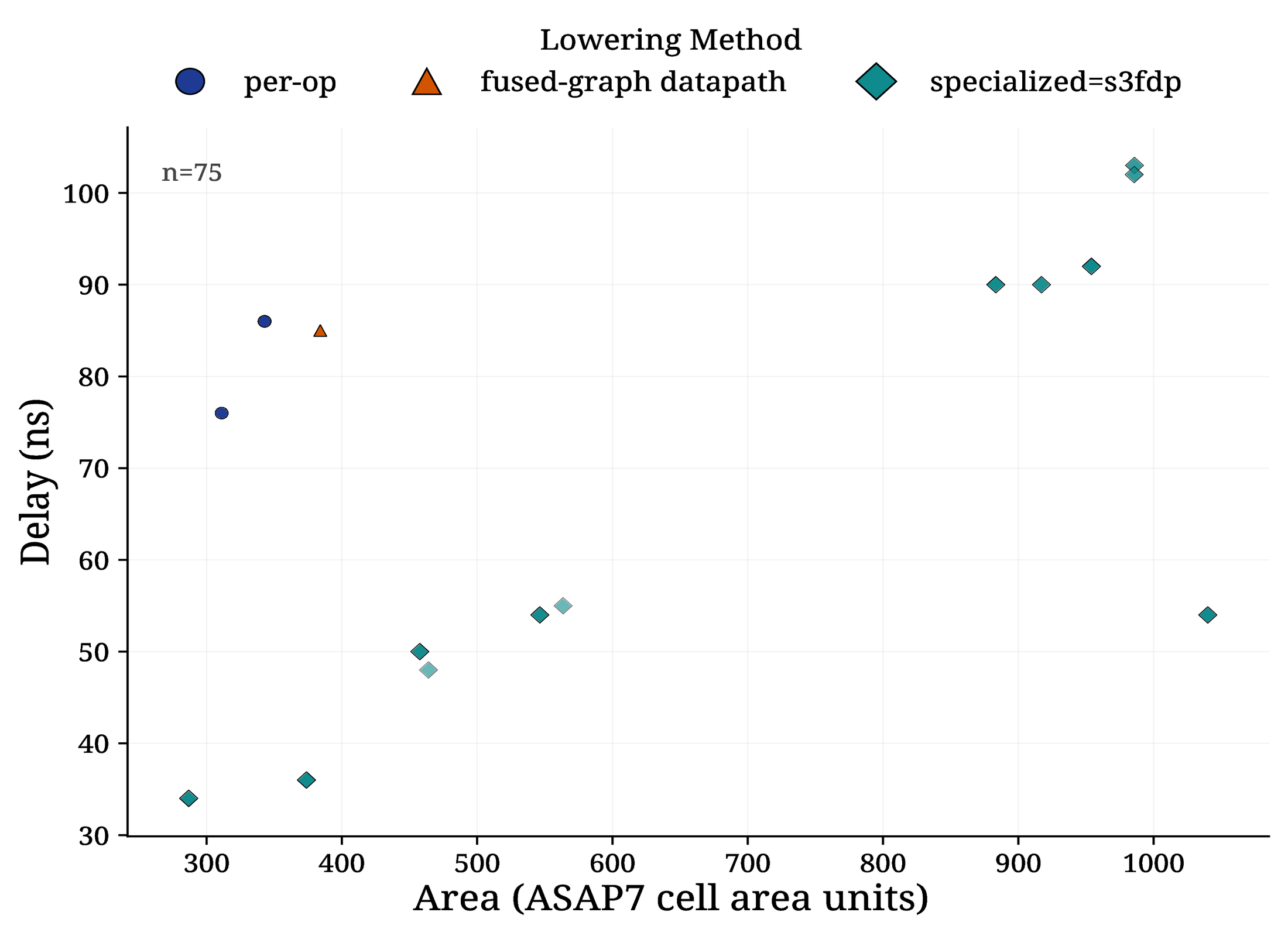
MatMul accumulation area versus delay

MatMul Accumulation. Area vs. Delay

Polybench GESUMMV-like

#map = affine_map<(d0, d1) -> (d0, d1)>
module {
  func.func @forward(%arg0: tensor<1x4xf32>) -> tensor<1x4xf32> {
    %mm = linalg.matmul ... -> tensor<1x4xf32>
    %out = linalg.generic ... ins(%mm, %arg0 : tensor<1x4xf32>, tensor<1x4xf32>) outs(%empty_out : tensor<1x4xf32>) {
    ^bb0(%mmv: f32, %in: f32, %acc: f32):
      %bias = arith.mulf %beta, %in : f32
      %res = arith.addf %mmv, %bias : f32
      linalg.yield %res : f32
    } -> tensor<1x4xf32>
    return %out : tensor<1x4xf32>
  }
}
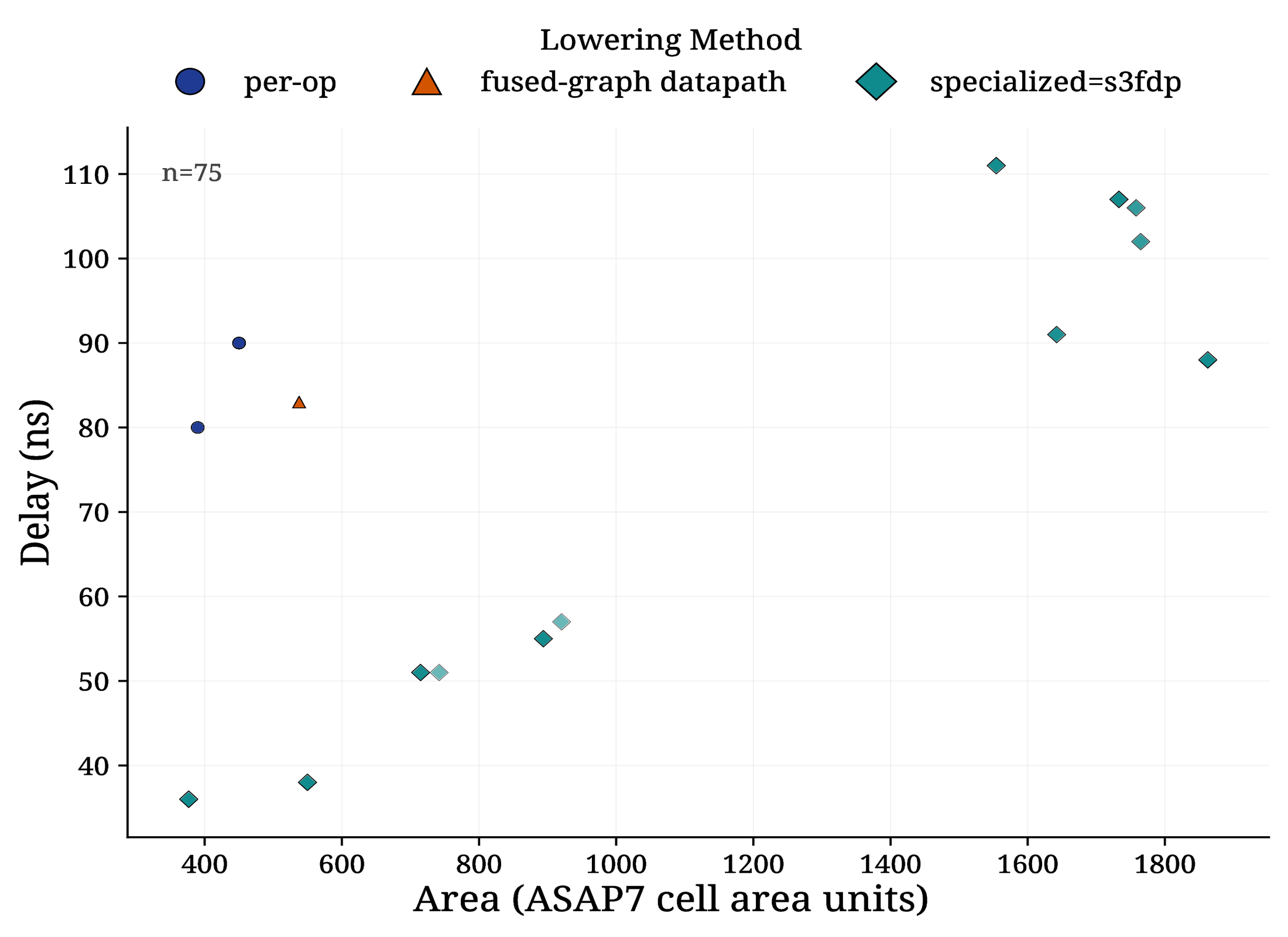
Polybench GESUMMV-like area versus delay

Polybench GESUMMV-Like. Area vs. Delay

DSP FIR accumulation

module {
  func.func @forward(%arg0: tensor<1x8xf32>) -> tensor<1x8xf32> {
    %w = arith.constant dense<...> : tensor<8x8xf32>
    %init = linalg.fill ins(%c0 : f32) outs(%empty : tensor<1x8xf32>) -> tensor<1x8xf32>
    %mm = linalg.matmul ins(%arg0, %w : tensor<1x8xf32>, tensor<8x8xf32>) outs(%init : tensor<1x8xf32>)
      -> tensor<1x8xf32>
    return %mm : tensor<1x8xf32>
  }
}
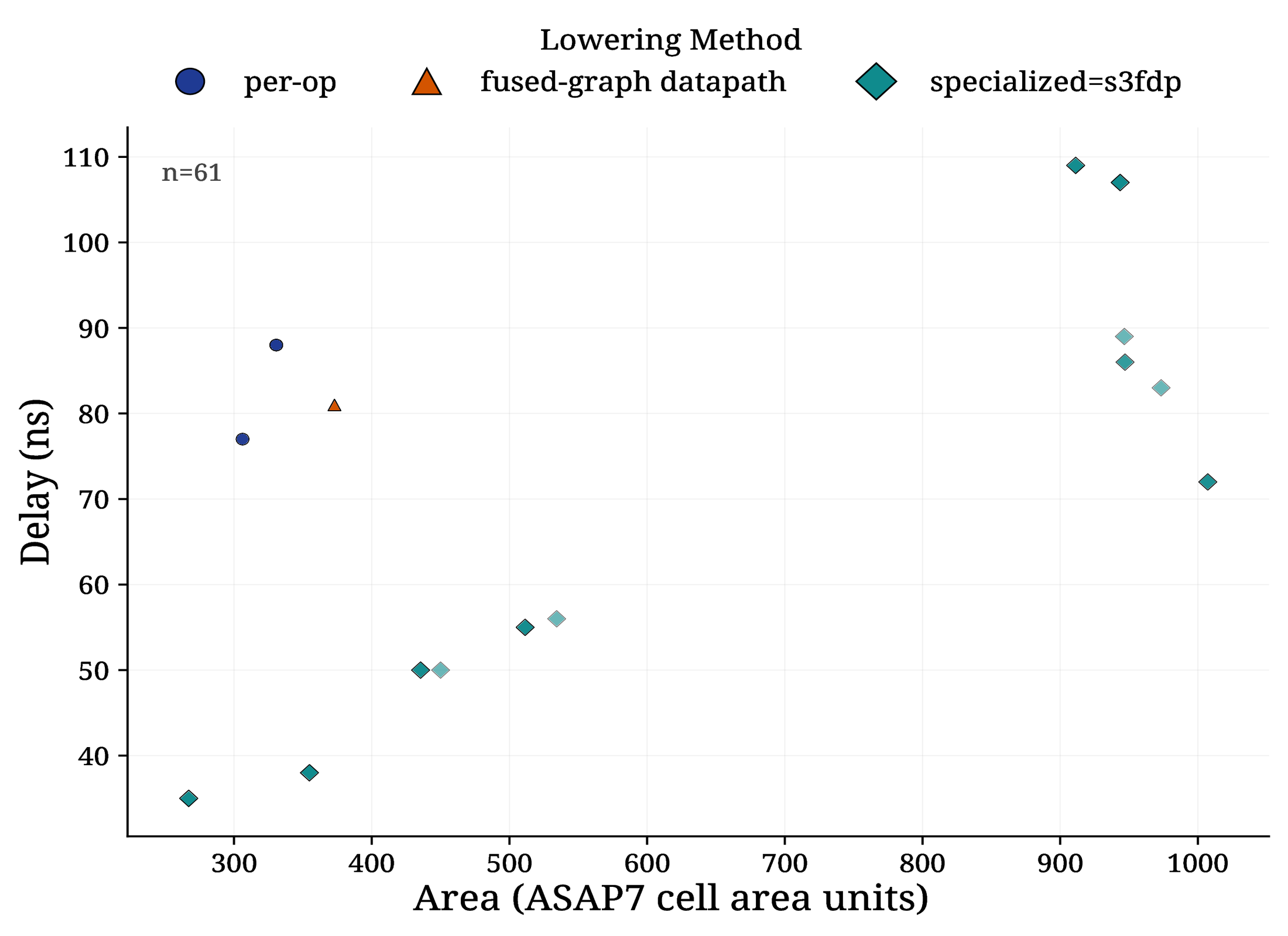
DSP FIR accumulation area versus delay

DSP FIR Accumulation. Area vs. Delay

Polybench SYRK-like

module {
  func.func @forward(%arg0: tensor<1x8xf32>) -> tensor<1x8xf32> {
    %w = arith.constant dense<...> : tensor<8x8xf32>
    %init = linalg.fill ins(%c0 : f32) outs(%empty : tensor<1x8xf32>) -> tensor<1x8xf32>
    %mm = linalg.matmul ins(%arg0, %w : tensor<1x8xf32>, tensor<8x8xf32>) outs(%init : tensor<1x8xf32>)
      -> tensor<1x8xf32>
    return %mm : tensor<1x8xf32>
  }
}
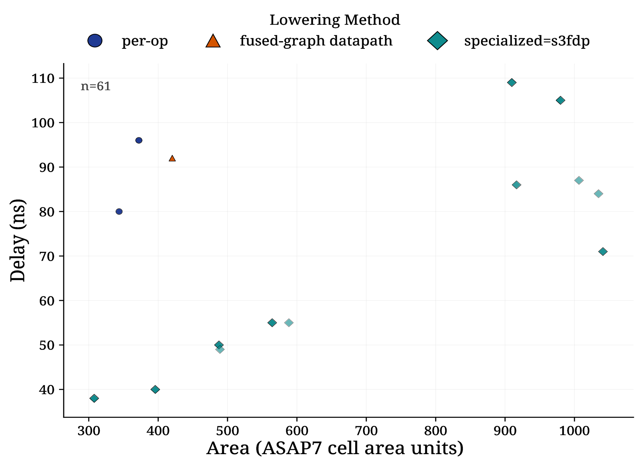
Polybench SYRK-like area versus delay

Polybench SYRK-Like. Area vs. Delay

Closing

CIRCT / LLVM commits

Accepted CIRCT pull request

Internal Emeraude-MLIR transforms pushed upstream.

Concluding remarks and future work

  • High level: broaden the polynomial approximation schemes.
  • Middle level: recognize and fuse more arithmetic patterns.
  • Low level: schedule comb graphs and materialize bit heaps.
  • Close the loop with cost models and design-space exploration.1 2
  • Upstream reusable components and open the research prototype.
  • Connect frontend, arithmetic, CIRCT, and EDA communities through explicit IR contracts.

1 Hanchen Ye et al., “ScaleHLS: A New Scalable High-Level Synthesis Framework on Multi-Level Intermediate Representation,” HPCA 2022.
2 Hanchen Ye and Deming Chen, “StreamTensor: Make Tensors Stream in Dataflow Accelerators for LLMs,” MICRO 2025.

Demo time :)

I will just execute a command while speaking

Thank you

Thank you

Q&A

Bibliography

  1. F. de Dinechin and M. Kumm, Application-Specific Arithmetic. Springer.
  2. B. Barbe, L. Ledoux, A. Volkova, and F. de Dinechin, “Reconfigurable constant multipliers: Hardware models, optimization algorithm and applications,” Microprocessors and Microsystems, p. 105270, 2026. doi:10.1016/j.micpro.2026.105270.
  3. L. Ledoux and M. Casas, “An Open-Source Framework for Efficient Numerically-Tailored Computations,” in 2023 33rd International Conference on Field-Programmable Logic and Applications (FPL), 2023, pp. 19–26. doi:10.1109/FPL60245.2023.00011.
  4. H. Ye et al., “ScaleHLS: A New Scalable High-Level Synthesis Framework on Multi-Level Intermediate Representation,” in 2022 IEEE International Symposium on High-Performance Computer Architecture (HPCA), 2022, pp. 741–755.

Bibliography

  1. H. Ye et al., “ScaleHLS: A New Scalable High-Level Synthesis Framework on Multi-Level Intermediate Representation,” in 2022 IEEE International Symposium on High-Performance Computer Architecture (HPCA), 2022, pp. 741–755. doi:10.1109/HPCA53966.2022.00060.
  2. H. Ye and D. Chen, “StreamTensor: Make Tensors Stream in Dataflow Accelerators for LLMs,” in Proceedings of the 58th IEEE/ACM International Symposium on Microarchitecture, MICRO ’25, Association for Computing Machinery, 2025, pp. 201–216. doi:10.1145/3725843.3762817.

Appendix

GDS cell usage

Cell usage by Category
Category Cells Count
Fill fillcap fill 10280
NAND nand2 nand4 nand3 2627
Combo Logic aoi21 oai21 oai22 oai31 aoi211 oai211 aoi22 oai32 oai221 aoi221 oai33 1645
Buffer clkbuf dlyb buf dlya 1258
Flip Flops dffq 1179
NOR nor2 nor4 nor3 xnor2 xnor3 1024
OR or2 or3 or4 xor2 xor3 1020
Clock clkinv 367
AND and2 and3 and4 323
Multiplexer mux2 316
Inverter inv 55

The complete precheck runs in GitHub Actions.

GDS precheck results

Tiny Tapeout Precheck Results
Check Result
Magic DRC
KLayout pin label overlapping drawing
KLayout zero area
KLayout Checks
Pin check
Boundary check
Power pin check
Layer check
Cell name check
Analog pin check

Many transforms from one Faust line of code passing all checks :)

References

Dean, Jeff, and Urs Hölzle. 2017. “Build and Train Machine Learning Models on Our New Google Cloud TPUs.” Google, May 17. https://blog.google/innovation-and-ai/infrastructure-and-cloud/google-cloud/google-cloud-offer-tpus-machine-learning/.
Dinechin, Florent de, and Martin Kumm. 2024. Application-Specific Arithmetic: Computing Just Right for the Reconfigurable Computer and the Dark Silicon Era. Springer Cham. https://doi.org/10.1007/978-3-031-42808-1.
Jouppi, Norman P., Doe Hyun Yoon, George Kurian, et al. 2020. “A Domain-Specific Supercomputer for Training Deep Neural Networks.” Communications of the ACM 63 (7): 67–78. https://doi.org/10.1145/3360307.
Ledoux, Louis. 2024. “Floating-Point Arithmetic Paradigms for High-Performance Computing: Software Algorithms and Hardware Designs.” PhD thesis, Universitat Politècnica de Catalunya.
Micikevicius, Paulius, Dusan Stosic, Neil Burgess, et al. 2022. FP8 Formats for Deep Learning.” arXiv Preprint arXiv:2209.05433, ahead of print. https://doi.org/10.48550/arXiv.2209.05433.
Mishchenko, Alan, Satrajit Chatterjee, and Robert K. Brayton. 2006. DAG-Aware AIG Rewriting: A Fresh Look at Combinational Logic Synthesis.” Proceedings of the 43rd Design Automation Conference, 532–35. https://doi.org/10.1145/1146909.1147048.
NVIDIA. 2022. NVIDIA Hopper Architecture in-Depth.” March 22. https://developer.nvidia.com/blog/nvidia-hopper-architecture-in-depth/.
Rupp, Karl. 2022. “50 Years of Microprocessor Trend Data.” https://github.com/karlrupp/microprocessor-trend-data.
Xilinx. 2019. “Virtex UltraScale+ VU19P FPGA Press Deck.” https://www.xilinx.com/publications/presentations/vu19p-press-deck.pdf.